Pricing CDOs using Intensity Gamma Approach
290 likes | 432 Views
Pricing CDOs using Intensity Gamma Approach. Christelle Ho Hio Hen Aaron Ipsa Aloke Mukherjee Dharmanshu Shah. Intensity Gamma. M.S. Joshi, A.M. Stacey “ Intensity Gamma: a new approach to pricing portfolio credit derivatives” , Risk Magazine, July 2006 Partly inspired by Variance Gamma

Pricing CDOs using Intensity Gamma Approach
E N D
Presentation Transcript
Pricing CDOs using Intensity Gamma Approach Christelle Ho Hio Hen Aaron Ipsa Aloke Mukherjee Dharmanshu Shah
Intensity Gamma • M.S. Joshi, A.M. Stacey “Intensity Gamma: a new approach to pricing portfolio credit derivatives”, Risk Magazine, July 2006 • Partly inspired by Variance Gamma • Induce correlation via business time
Business time Calendar time Business time vs. Calendar time
Calibration Parameter guess Survival Curve Construction 6mo 1y 2y .. 5y name1 . name2 . . name125 IG Default Intensities CDS spreads Tranche pricer Default time calculator Business time path generator 0-3% … 3-6% … 6-9% … . . Market tranche quotes Objective function NO Err<tol? YES Block diagram
Advantages of Intensity Gamma • Market does not believe in the Gaussian Copula • Pricing non-standard CDO tranches • Pricing exotic credit derivatives • Time homogeneity
The Survival Curve • Curve of probability of survival vs time • Jump to default = Poisson process P(λ) • Default = Cox process C(λ(t)) • Pr (τ > T) = exp[ ] • Intensity vs time – λT1, λT2, λT3….. for (0,T1), (0,T2), (0,T3)
Bootstrapping the Survival Curve • Assume a value for λT1 • X(0,T1) = exp(-λT1 . T1) • Price CDS of maturity T1 • Use a root solving method to find λT1 • Assume a value for λT2 • Now X(0,T2) = X(0,T1) * exp(-λT2(T2-T1)) • Price CDS of maturity T2 • Use root solving method to find λT2 • Keep going on with T3, T4….
Constructing a Business Time Path • Business time modeled as two Gamma Processes and a drift.
Constructing a Business Time Path • Characteristics of the Gamma Process • Positive, increasing, pure jump • Independent increments are Gamma distributed:
Constructing a Business Time Path • Series Representation of a Gamma Process (Cont and Tankov) • T,V are Exp(1), No Gamma R.V’s Req’d.
Constructing a Business Time Path Truncation Error Adjustment
Constructing a Business Time Path Truncation Error Adjustment
Constructing a Business Time Path • Test Effect of Estimating Truncation Error in Generating 100,000 Gamma Paths • 1. Set Error = .001, no adjustment • Computation Time = 42 Seconds • 2. Set Error = 0.05 and apply adjustment • Computation Time = 34 seconds
Constructing a Business Time Path • Testing Business Time Paths • Given drift a = 1, Tenor = 5, 100,000 paths Mean = 63.267 +/- 0.072 Expected Mean = 63.333
Constructing a Business Time Path …Testing Business Time Path Continued Variance = 522.3 Expected Variance = 527.8
IG Forward Intensities ci(t) • In IG model survival probability decays with business time • Inner calibration: parallel bisection • Note that one parameter redundant
Default Times from Business Time • Survival Probability: • Default Time:
Tranche pricer • Calculate cashflows resulting from defaults • Validation: reprice CDS (N=1) EDU>> roundtriptest(100,100000); closed form vfix = 0.0421812, vflt = 0.0421812 Gaussian vfix = 0.0422499, vflt = 0.0428865 IG vfix = 0.0429348, vflt = 0.0422907 input spread = 100, gaussian spread = 101.507, IG spread = 98.4998 • Validation: recover survival curve
A Fast Approximate IG Pricer • Constant default intensities λi • Probability of k defaults given business time IT • Price floating and fixed legs by integrating over distribution of IT
Fast IG Approximation Comparison Tranche Fast IG Full IG 0-3% 1429 1778 3-7% 135 187 7-10% 14 29 10-15% 1 5 15-30% 0 0
Fast Approx – Both Constant λi Tranche Fast IG Full IG 0-3% 1429 1573 3-7% 135 133 7-10% 14 13 10-15% 1 1 15-30% 0 0
Fast Approx – Const λi, Uniform Default Times Tranche Fast IG Full IG 0-3% 1584 1573 3-7% 144 133 7-10% 14 13 10-15% 1 1 15-30% 0 0
Calibration • Unstable results => need for noisy optimization algorithm. • Unknown scale of calibration parameters => large search space. • Long computation time => forbids Genetic Algorithm Simulated Annealing
Calibration • Redundant drift value => set a = 1 • Two Gamma processes: = 0.2951 = 0.2838 = 0.0287 = 0.003
Future Work • Performance improvements • Use “Fast IG” as Control Variate • Quasi-random numbers • Not recommended for pricing different maturities than calibrating instruments • Stochastic delay to default • Business time factor models