Example
This article explores the directionality of analysis in flow functions and the precision of dataflow analysis. It discusses the theory and examples of backward analyses, the issues of precision loss, and the concept of MOP (Meet Over all Paths) versus dataflow. It also examines distributive problems and how they affect the accuracy of dataflow analysis.

Example
E N D
Presentation Transcript
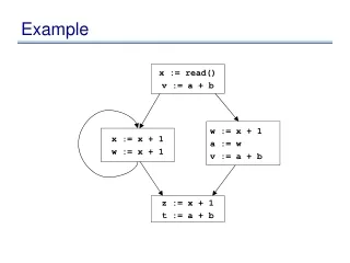
Example x := read() v := a + b w := x + 1 a := w v := a + b x := x + 1 w := x + 1 z := x + 1 t := a + b
Direction of analysis • Although constraints are not directional, flow functions are • All flow functions we have seen so far are in the forward direction • In some cases, the constraints are of the form in = F(out) • These are called backward problems. • Example: live variables • compute the set of variables that may be live
Live Variables • A variable is live at a program point if it will be used before being redefined • A variable is dead at a program point if it is redefined before being used
Example: live variables • Set D = • Lattice: (D, v, ?, >, t, u) =
Example: live variables • Set D = 2 Vars • Lattice: (D, v, ?, >, t, u) = (2Vars, µ, ; ,Vars, [, Å) in Fx := y op z(out) = x := y op z out
Example: live variables • Set D = 2 Vars • Lattice: (D, v, ?, >, t, u) = (2Vars, µ, ; ,Vars, [, Å) in Fx := y op z(out) = out – { x } [ { y, z} x := y op z out
Example: live variables x := 5 y := x + 2 y := x + 10 x := x + 1 ... y ...
Example: live variables x := 5 y := x + 2 y := x + 10 x := x + 1 ... y ... How can we remove the x := x + 1 stmt?
Revisiting assignment in Fx := y op z(out) = out – { x } [ { y, z} x := y op z out
Revisiting assignment in Fx := y op z(out) = out – { x } [ { y, z} x := y op z out
Theory of backward analyses • Can formalize backward analyses in two ways • Option 1: reverse flow graph, and then run forward problem • Option 2: re-develop the theory, but in the backward direction
Precision • Going back to constant prop, in what cases would we lose precision?
Precision • Going back to constant prop, in what cases would we lose precision? if (...) { x := -1; } else x := 1; } y := x * x; ... y ... if (p) { x := 5; } else x := 4; } ... if (p) { y := x + 1 } else { y := x + 2 } ... y ... x := 5 if (<expr>) { x := 6 } ... x ... where <expr> is equiv to false
Precision • The first problem: Unreachable code • solution: run unreachable code removal before • the unreachable code removal analysis will do its best, but may not remove all unreachable code • The other two problems are path-sensitivity issues • Branch correlations: some paths are infeasible • Path merging: can lead to loss of precision
MOP: meet over all paths • Information computed at a given point is the meet of the information computed by each path to the program point if (...) { x := -1; } else x := 1; } y := x * x; ... y ...
MOP • For a path p, which is a sequence of statements [s1, ..., sn] , define: Fp(in) = Fsn( ...Fs1(in) ... ) • In other words: Fp = • Given an edge e, let paths-to(e) be the (possibly infinite) set of paths that lead to e • Given an edge e, MOP(e) = • For us, should be called JOP (ie: join, not meet)
MOP vs. dataflow • MOP is the “best” possible answer, given a fixed set of flow functions • This means that MOP v dataflow at edge in the CFG • In general, MOP is not computable (because there can be infinitely many paths) • vs dataflow which is generally computable (if flow fns are monotonic and height of lattice is finite) • And we saw in our example, in general,MOP dataflow
MOP vs. dataflow • However, it would be great if by imposing some restrictions on the flow functions, we could guarantee that dataflow is the same as MOP. What would this restriction be? Dataflow MOP x := -1; y := x * x; ... y ... x := 1; y := x * x; ... y ... x := -1; x := 1; Merge y := x * x; ... y ... Merge
MOP vs. dataflow • However, it would be great if by imposing some restrictions on the flow functions, we could guarantee that dataflow is the same as MOP. What would this restriction be? • Distributive problems. A problem is distributive if: 8 a, b . F(a t b) = F(a) t F(b) • If flow function is distributive, then MOP = dataflow
Summary of precision • Dataflow is the basic algorithm • To basic dataflow, we can add path-separation • Get MOP, which is same as dataflow for distributive problems • Variety of research efforts to get closer to MOP for non-distributive problems • To basic dataflow, we can add path-pruning • Get branch correlation • To basic dataflow, can add both: • meet over all feasible paths