Inference about the Slope and Intercept

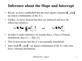
1. Inference about the Slope and Intercept • Recall, we have established that the least square estimates and are linear combinations of the Yi’s. • Further, we have showed that they are unbiased and have the following variances • In order to make inference we assume that εi’s have a Normal distribution, that is εi ~ N(0, σ2). • This in turn means that the Yi’s are normally distributed. • Since both and are linear combination of the Yi’s they also have a Normal distribution. STA302/1001 - week 4

2. Inference for β1 in Normal Error Regression Model • The least square estimate of β1 is , because it is a linear combination of normally distributed random variables (Yi’s) we have the following result: • We estimate the variance of by S2/SXX where S2 is the MSE which has n-2 df. • Claim: The distribution of is t with n-2 df. • Proof: STA302/1001 - week 4

3. Tests and CIs for β1 • The hypothesis of interest about the slope in a Normal linear regression model is H0: β1 = 0. • The test statistic for this hypothesis is • We compare the above test statistic to a t with n-2 df distribution to obtain the P-value…. • Further, 100(1-α)% CI for β1 is: STA302/1001 - week 4

4. Important Comment • Similar results can be obtained about the intercept in a Normal linear regression model. • See the book for more details. • However, in many cases the intercept does not have any practical meaning and therefore it is not necessary to make inference about it. STA302/1001 - week 4

5. Example • We have Data on Violent and Property Crimes in 23 US Metropolitan Areas.The data contains the following three variables: violcrim = number of violent crimes propcrim = number of property crimes popn = population in 1000's • We are interested in the relationship between the size of the city and the number of violent crimes…. STA302/1001 - week 4

6. Comments Regarding the Crime Example • A regression model fit to data from all 23 cities finds a statistically significant linear relationship between numbers of violent crimes in American cities and their populations. • For each increase of 1,000 in population, the number of violent crimes increases by 0.1093 on average. 48.6% of the variation in number of violent crimes can be explained by its relationship with population. • Because these data are observational, i.e. collected without experimental intervention, it cannot be said that larger populations cause larger numbers of crimes, but only that such an association appears to exist. • However, this linear relationship is mostly determined by New York City whose population and number of violent crimes are much larger than any other city, and thus accounts for a large fraction of the variation in the data. When New York is removed from the analysis there is no longer a statistically significant linear relationship and the linear relationship with population explains less than 9% of the variation in number of violent crimes. STA302/1001 - week 4

7. Bivariate Normal Distribution • X and Y are jointly normally distributed if their joint density is where - ∞ < x < ∞ and - ∞ < y < ∞. • Can show that the marginal distributions are: and ρ is the correlation between X and Y, i.e., STA302/1001 - week 4

8. Properties of Bivariate Normal Distribution • It can be shown that the conditional distribution of Y given X = x is: • Linear combinations of X and Y are normally distributed. • A zero covariance between any X and Y implies that they are statistically independent. Note that this is not true in general for any two random variables. STA302/1001 - week 4

9. Sample Correlation • If X and Y are random variables, and we would like a symmetric measure of the direction and strength of the linear relationship between them we can use correlation. • Based on n observed pairs (xi , yi) i =1,…,n, the estimate of the population correlation ρ is the Pearson’s Product-Moment Correlation given by • It is the MLE of ρ. STA302/1001 - week 4

10. Facts about r • It measures the strength of the linear relationship between X and Y. • It is distribution free. • r is always a number between –1 and 1. • r = 0 indicates no linear association. • r = –1 or 1 indicates that the points fall perfectly on a straight line with negative slope. • r = 1 or 1 indicates that the points fall perfectly on a straight line with positive slope. • The strength of the linear relationship increases as r moves away from 0. STA302/1001 - week 4

11. STA302/1001 - week 4

12. Relationship between Regression and Correlation STA302/1001 - week 4