Download

1 / 31
480 likes | 1.04k Views
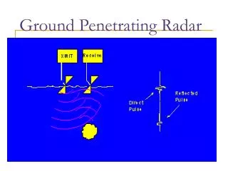
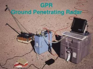
Ground Penetrating Radar GPR. Noggin Plus 250 Configuration. DVL (Digital Video Logger) . cable. Battery. Odometer. Smart Cart. Noggin Plus 250 . Trade-Off Resolution and Antenna Frequency Low frequency Antenna High frequency Antenna

E N D
Noggin Plus 250 Configuration DVL (Digital Video Logger) cable Battery Odometer Smart Cart Noggin Plus 250
Trade-Off Resolution and Antenna Frequency Low frequency AntennaHigh frequency Antenna Long Wavelength Short Wavelength Decreased Resolution Increased Resolution Increased Depth Penetrating Decreased Depth Penetrating Increased size and weight Decreased size and weight
Values of conductivity, relative permittivity, and approximate velocity. (Schultz (2002), Milsom, (2003), Davis and Annan, (1998), and Conyers, (2004)) (After Burger, H. R., 2006).
Equation used to determine the depth, d, where c is the speed of light in a vacuum, is the probably one permeability, and is the relative permittivity.
300 cm GPR Antenna z x 250 cm Dry Sand (r =5, σ =10-5 S/m) (r = 30, σ = 10-3 S/m) (r = 19, σ = 0.021 S/m) Saturated Sand/Clay Limestone (r = 7, σ = 10-9 S/m) The model schematic diagram that is used in synthetic simulation of the GPR data. For model 1, the middle layer is saturated sand and it is saturated clay for model 2. r is permittivity and σ is conductivity y
The top diagram represents the signal for model 1 (the second layer is saturated sand). The bottom diagram is the signal for model 2 (the second layer is saturated clay). The 1st arrow points at the reflection from dry sand-saturated sand (saturated clay for model 2) discontinuity. The 2nd arrow points at the reflection from the saturated sand (saturated clay for model 2)–limestone discontinuity. The 3rd arrow points at the reflection from the bottom of the model
Schematic diagram of the model geometry used to simulate GPR data to model two-limestone block
The diagram represents the signal for model 1. The 1st arrow in this waveform points at the onset time of the reflections from the dry sand-the first limestone block discontinuity, and the 2nd arrow points at the onset of the reflections from the second limestone block-dry sand discontinuity. The 3rd arrow indicates the arrival of reflection from the bottom of the model
Schematic diagram of the model geometry used to simulate GPR data to model vertical and reverse faults
The diagram represents the signal for 2nd and 3rd models. The 1st arrow in these two waveforms points at the onset time of the reflections from the dry sand-the first limestone half block discontinuities, and the 2nd arrow points at the onset of the reflections from dry sand-the second limestone half block discontinuity. The 3rd arrow indicates the arrival of reflection from the bottom of the model
Radar Data Processing
Example of GPR profile before and after zero time processing: (top) before processing and (bottom) after processing.
Example of GPR profile before and after horizontal filter and low 500 and high 300 filtering: (top) before processing and (bottom) after processing.
Example of GPR profile before and after background removal processing: (top) before processing and (bottom) after processing.
Example of GPR profile before and after migration processing: (top) before processing and (bottom) after processing.
Lap Experiments and Campus Field work Using GPR Technique
Time (ns) 4 cm Sand 5 cm Concrete 20 Cm Sand 54 cm Concrete 5 cm Sand 20 cm 130 cm
Time (ns) 4 cm Sand Sand Concrete 5 cm 20 cm 54 cm 5 cm Concrete 20 cm 130 cm
Detection of cavity under Hot Mix Asphalt pavement (top left image). Top right image shows the survey profiles (arrows). 3D GPR image before the cavity excavation (top block) and after the excavation (middle block). Contact between the aggregate and the soil is shown as black line (top block). Blue line in the lower block represents the reflections from the contact between the HMA and the aggregates
Conclusions • Computer based simulations and controlled laboratory experimentation show that GPR can map variation in lithology and structural setting.
Thank You Questions