Modeling Carbon Flux and Environmental Factors: A Comprehensive Analysis of Seasonal Dynamics
590 likes | 714 Views
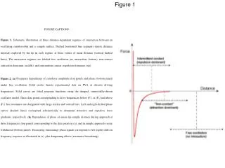
This study presents a detailed analysis of carbon dioxide fluxes ([umoleCO2/m²/s]) across different seasons, utilizing various models to assess the influence of temperature and soil moisture on carbon balance. By comparing model predictions to observed data from 1992-2000, the research highlights improvements in model accuracy when incorporating phenological aspects. The paper also examines the relationship between precipitation, water vapor flux, and potential recharge, emphasizing the significance of seasonal variations in environmental conditions on carbon dynamics in ecosystems.

Modeling Carbon Flux and Environmental Factors: A Comprehensive Analysis of Seasonal Dynamics
E N D
Presentation Transcript
Figure 3 a2 [umoleCO2/m2/s/degC] a1 [umoleCO2/m2/s] a3 [umoleCO2/m2/s] -a3/a4 [umoleCO2/m2/s/umole-photon]
Figure 4 Model-0 parameter a1 vs. mean Tair Early summer 5 late spring Mid-summer 4 late summer early spring a1 [umoleCO2/m2/s] 3 late fall early fall 2 winter 0 5 10 15 Ta5mean [degC]
Figure 5 Precipitation - Water Vapor Flux = Potential Recharge / Total Loss TL ppt > Fh2o Fh2o > ppt PR surface layer Z = ZTOP SL = min{TL*(sfcM), sfc} If und > und.thresh UL = min{TL - SL , und} Else UL = buffer*(TL - SL) wctop SR = min{*PR, wcbot - sfc} UR = min{PR - SR, wctop - und} RO = PR - SR - UR wcbot under layer Z = ZBOT
1.0 hour season 0.8 0.6 soil moisture R2 phenology 0.4 0.2 0.0 early spring late spring early fall early mid late late fall winter summer Figure 19 Statistical model R2 for hour and season time scales. Arrows and highlighted markers show the increase in model skill upon inclusion of phenology and soil moisture.
Fig 20a 1992-2000 Model-0 vs. Observed DOY 341-100 hour(5-day) time scale 20 R2 = 0 RMSE = 1.24 a0 = -0.72 +/- 0.41 a1 = 1.59 +/- 0.33 15 10 obs NEE 5 0 -5 -5 0 5 10 15 20 pred NEE NEE in units of [umoleCO2/m2/s]
Fig 20b NEE in units of [umoleCO2/m2/s]
Fig 21a NEE in units of [umoleCO2/m2/s]
Fig 21b NEE in units of [umoleCO2/m2/s]
Figure 24 Model-0 = black Model-0 + wind direction = red NEE in units of [umoleCO2/m2/s]
1992-2000 Model-0/0B vs. Observed DOY 206 - 250 1992-2000 Model-0/0C vs. Observed DOY 206 - 250 month time scale month time scale 99 99 M0 -3.0 99 99 M0B M0 -3.0 M0C 92 92 -3.5 92 92 -3.5 98 98 00 00 98 98 00 00 -4.0 obs NEE -4.0 obs NEE 95 95 95 95 94 94 -4.5 94 94 -4.5 97 97 96 96 -5.0 97 97 96 96 -5.0 -5.5 93 93 -5.5 93 93 -5.5 -5.0 -4.5 -4.0 -3.5 -3.0 -5.5 -5.0 -4.5 -4.0 -3.5 -3.0 pred NEE pred NEE FIGURE 25
1992-2000 Mid-summer Model-I NEE vs. Observed NEE R2 = 0.92 RMSE = 0.23 a0 = 0.18 +/- 0.48 10 a1 = 0.85 +/- 0.63 1:1 0 Observed NEE -10 best fit -20 -30 -30 -20 -10 0 10 predicted NEE Figure 28a Figure 28a. 1992-2000 Mid-summer NEE. Five-day aggregates of Model-I predicted NEE vs. Observed NEE.
1992-2000 Mid-summer NEE Model-I vs. Observed R2 = 0.47 RMSE = 0.23 a0 = 0.18 +/- 0.48 -1 a1 = 0.85 +/- 0.63 -2 -3 Observed NEE -4 -5 -6 -6 -5 -4 -3 -2 -1 predicted NEE Figure 28b Figure 28b. 1992-2000 Mid-summer daily mean NEE. Model-I predicted NEE vs. Observed NEE. Data uses Five-day aggregates. 1:1 best fit
Figure 28c 1992-2000 Mid-summer NEE. Model-I vs. Observed Model-I fit statistics 99 99 Figure 28c. 1992-2000 Mid-summer seasonal mean NEE. Model-0 (black numbers) and Model-I (red numbers) predicted NEE vs. Observed NEE. Data uses five-day aggregates. R2 = 0.76 -3.0 RMSE = 0.23 a0 = 0.18 +/- 0.48 a1 = 0.85 +/- 0.63 -3.5 92 92 98 98 Observed NEE 00 00 95 95 -4.0 94 94 -4.5 96 96 97 97 93 93 -4.5 -4.0 -3.5 -3.0 Predicted NEE
Figure 29a 10 5 0 -10 -20 208 213 218 10 5 0 -5 -15 223 228 233 10 5 0 -10 -20 238 243 248 1999 Mid-summer NEE Figure29a. 1999 Mid-summer five-day aggregates of observed, Model-0, and Model-I NEE. Observed (empty squares), Model-0 (red squares), Model-I (blue diamonds)
Figure 29b 10 0 -10 -20 208 213 218 5 0 -5 -10 -15 -20 223 228 233 5 0 -5 -10 -20 238 243 248 1994 Mid-summer NEE Figure 29b. 1994 Mid-summer five-day aggregates of observed, Model-0, and Model-I NEE. Observed (empty squares), Model-0 (red squares), Model-I (blue diamonds)