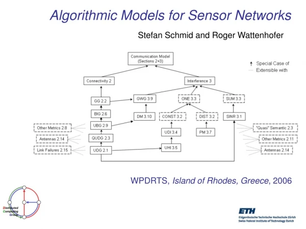
Algorithmic Models for Sensor Networks
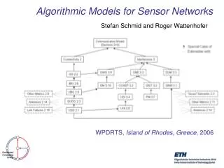
Stefan Schmid and Roger Wattenhofer. Algorithmic Models for Sensor Networks. WPDRTS, Island of Rhodes, Greece , 2006. Algorithmic Models. Why are models needed? - Formal proofs of correctness, efficiency, real-time guarantees, … - Common basis to compare results?.

Algorithmic Models for Sensor Networks
E N D
Presentation Transcript
Stefan Schmid and Roger Wattenhofer Algorithmic Models for Sensor Networks WPDRTS, Island of Rhodes, Greece, 2006
Algorithmic Models • Why are models needed? - Formal proofs of correctness, efficiency, real-time guarantees, … - Common basis to compare results? A typical problem in sensor networks: Find the destination! source destination Stefan Schmid, ETH Zurich @ WPDRTS 2006
Finding a Destination Stefan Schmid, ETH Zurich @ WPDRTS 2006
Finding a Destination Efficiently: Backbone Stefan Schmid, ETH Zurich @ WPDRTS 2006
Backbone • Idea: Some nodes become backbone nodes (gateways). Each node can access and be accessed by at least one backbone node. • Routing: • If source is not agateway, transmitmessage to gateway • Gateway acts asproxy source androutes message onbackbone to gatewayof destination. • Transmission gatewayto destination. Stefan Schmid, ETH Zurich @ WPDRTS 2006
(Connected) Dominating Set • A Dominating Set DS is a subset of nodes such that each node is either in DS or has a neighbor in DS. • A Connected Dominating Set CDS is a connected DS, that is, there is a path between any two nodes in CDS that does not use nodes that are not in CDS. • A CDS is a good choicefor a backbone. • It might be favorable tohave few nodes in the CDS. This is known as theMinimum CDS problem. Stefan Schmid, ETH Zurich @ WPDRTS 2006
A Famous Dominating Set… Stefan Schmid, ETH Zurich @ WPDRTS 2006
Algorithm 1 Input: Local Graph Fractional Dominating Set Dominating Set Connected Dominating Set 0.2 0.2 0 0.5 0.3 0 0.8 0.3 0.5 0.1 0.2 Phase B: Probabilistic algorithm Phase C: Connect DS by “tree” of “bridges” Phase A: Distributed linear program Stefan Schmid, ETH Zurich @ WPDRTS 2006
Algorithm 1: Phase A Stefan Schmid, ETH Zurich @ WPDRTS 2006
Algorithm 1: Phase B Each node applies the following algorithm: • Calculate (= maximum degree of neighbors in distance 2) • Become a dominator (i.e. go to the dominating set) with probability • Send status (dominator or not) to all neighbors • If no neighbor is a dominator, become a dominator yourself Highest degree in distance 2 From phase A Stefan Schmid, ETH Zurich @ WPDRTS 2006
Algorithm 2: Idea transmission radius Stefan Schmid, ETH Zurich @ WPDRTS 2006
Algorithm 2 • Beacon your position • If, in your virtual grid cell, you are the node closest to the center of the cell, then join the DS, else do not join. • That’s it. Stefan Schmid, ETH Zurich @ WPDRTS 2006
Algorithm 1 Algorithm computes DS k2+O(1) transmissions/node O(O(1)/klog ) approximation Quite complex! Performance OK Algorithm 2 Algorithm computes DS 1transmission/node O(1) approximation Easy! Performance great! Comparison General Graph! No Position Information! Unit Disk Graph Only! Requires GPS Device! The model determines the distributed complexity of clustering Stefan Schmid, ETH Zurich @ WPDRTS 2006
Time: Approximation: Relation Between Algorithms and Models Bounded Independence General Graph UBG Distances UDG, no Distances UDG Distances UDG GPS too optimistic too pessimistic too simplistic too realistic Message Passing Models Physical Signal Propagation Unstructured Radio Network Model Radio Network Model Stefan Schmid, ETH Zurich @ WPDRTS 2006
Let‘s Talk about Models! • Why models for sensor networks? • Allows precise evaluation of algorithms • Analysis of correctness and efficiency (proofs) • Goal of model designer? • Simplifications and abstractions • But close to reality! Stefan Schmid, ETH Zurich @ WPDRTS 2006
Let’s Talk about Models! • Model for what? • Connectivity • Interference • Algorithm type • Node distribution • Energy consumption • etc.! Stefan Schmid, ETH Zurich @ WPDRTS 2006
Let’s Talk about Models! • Algorithmic models often inspired by • “Connections” => Graph Theory • Transmission ranges, interference, … => Geometry • Goal of our paper: • Survey of simple algorithmic models • “higher level abstractions“ We ask: - How are models related to each other? - When should which model be preferred? Stefan Schmid, ETH Zurich @ WPDRTS 2006
Connectivity: Unit Disk Graph Which nodes are adjacent to a given node v? • Example: Unit Disk Graph (UDG) • Classic Model from computational geometry • {u,v} 2 E , |u,v| · 1 • Pro • Very simple • Analytically tractable • Realistic for unobstructed environments • Contra • Too simple • Not realistic for inner-city networks with many buildings etc. Stefan Schmid, ETH Zurich @ WPDRTS 2006
R R Connectivity: Unit Disk Graph Unit Disk Graph Stefan Schmid, ETH Zurich @ WPDRTS 2006
Connectivity: Quasi Unit Disk Graph • More realistic: Quasi UDG (QUDG) • two radii • {u,v} 2 E , |u,v| · • {u,v} 2 E , |u,v| > 1 • otherwise: It depends! • It depends… • … on an adversary, • … on probabilistic model, • etc.! Advantage: More flexible and realistic than UDG! Stefan Schmid, ETH Zurich @ WPDRTS 2006
Connectivity: Drawbacks of QUDG • How realistic is QUDG? • if there is a wall… • … u and v can be close but not adjacent • => QUDG model requires very small • However, although if there are walls, connectivity typically still adheres to certain geometric constraints! • Resort to general connectivity graphs too pessimistic! • Observation: Even in complex environments, the neighbors of a node are often also neighboring (cf wall example) - Motivation for Bounded Independence Graph! Stefan Schmid, ETH Zurich @ WPDRTS 2006
Connectivity: Bounded Independence Graph Bounded Independence Graph (BIG) • Size of any independent set grows polynomially with the hop distance r - typically: in O(rc) for constant c¸ 2 Stefan Schmid, ETH Zurich @ WPDRTS 2006
Connectivity : Unit Ball Graph Finally, there are many interesting UDG generalizations • Example: Unit Ball Graph (UBG) • Nodes are assumed to form a doubling metric • The set of nodes at distance r of a node u can be covered by a constant number of balls of radius r/2 around other nodes, for all r • i.e., Bu(r) µi=1…c Bui(r/2), 8 r Stefan Schmid, ETH Zurich @ WPDRTS 2006
Connectivity: Unit Ball Graph S 1 1 1 Stefan Schmid, ETH Zurich @ WPDRTS 2006
Connectivity Put into Perspective (1) • Fact: UDG is a QUDG • = 1 UBG However, in the QUDG with constant , the set of nodes in radius r can always be covered by a constant number of balls of radius r/2 and hence: QUDG Fact: QUDG is a UBG UDG Stefan Schmid, ETH Zurich @ WPDRTS 2006
Connectivity Put into Perspective (2) • Fact: The UBG is a BIG. - The size of the independent sets of any UBG is polynomially bounded. GG BIG Fact: A BIG is of course a special kind of a general graph (GG). UBG QUDG UDG Stefan Schmid, ETH Zurich @ WPDRTS 2006
More Models! • Interference - Which senders can disturb the reception of which other peers? Node distribution vs vs • Location information - GPS / Galileo device, etc.? Etc.! Stefan Schmid, ETH Zurich @ WPDRTS 2006
Choice of Model (1) Which model to choose? Stefan Schmid, ETH Zurich @ WPDRTS 2006
Choice of Model (2) Which model to choose? General Graph UDG too optimistic too pessimistic Unit Ball Graph Quasi UDG Bounded Independence 1 d Stefan Schmid, ETH Zurich @ WPDRTS 2006
Choice of Model (3) Note: An algorithm which is correct in a “higher” model is also correct in a “lower” model in our figure. Robustness and correctness properties of an algorithm should be proven in a model as high as possible! For efficiency considerations, however, a less conservative and more idealistic model might be fine! And: Study of simpler models might give insights into how algorithms for general model could look like! Stefan Schmid, ETH Zurich @ WPDRTS 2006
Conclusion • Models… • … influence design, performance, correctness of algorithms! • … are more sophisticated than some years ago. • … still require lot of research. • … are not even completely known by experts! • … raise interesting questions of how they are related! • Our paper… • … surveys models for connectivity, interference, etc. • … mostly simplistic models (“high-level”) only. • … a first step to put things into perspective! Stefan Schmid, ETH Zurich @ WPDRTS 2006
Thank you for your attention! Stefan Schmid, ETH Zurich @ WPDRTS 2006
Questions? / Feedback? Stefan Schmid, ETH Zurich @ WPDRTS 2006