Download
1 / 37
370 likes | 571 Views
EE442 --Digital Signals and Filtering, Winter 2004 (MWF, 9:30-10:20 am, EE1 045). Prof. Jenq-Neng Hwang, (hwang@ee.washington.edu) Office Hours (EE M426): Mon,Wed,Th 1:30 -- 2:30 pm

E N D
EE442 --Digital Signals and Filtering, Winter 2004(MWF, 9:30-10:20 am, EE1 045) • Prof. Jenq-Neng Hwang, (hwang@ee.washington.edu) • Office Hours (EE M426): Mon,Wed,Th 1:30 -- 2:30 pm • Two courses sequence: EE442 (signal transforms and filterings) and EE443 (applications and real-time DSP microprocessor design) • The prerequisite for this course is EE341 • discrete time signals and LTI systems • Fourier transforms (continuous-time and discrete-time) • Laplace transform and Z-transform • TA: Somsak Sukittanon (ssukitta@u.washington.edu) • TA Office Hours (EE 423) Tue,Fri 1:30 – 3:00 pm • Credits: 1 Science and 2 Design
Goals and Grading • Goals: to provide students with the fundamental knowledge of digital filter characteristics, design principles and design specifications. Applications to adaptive filtering and speech processing are also introduced. • Grading:Matlab Labs: 24%, 1st Midterm Exam.: 32%, 2nd Midterm Exam: 44% • Textbook: Vinay K. Ingle and John G. Proakis, Digital Signal Processing using Matlab, 2nd Edition, Brooks/Cole Publishing, 2000. • Reference: additional materials related to DSP applications.
Topics and Schedules • Review of Discrete-Time Fourier Transform (DTFT) and Z Transform --- 1 week (chapters 1,2,3,4) • Review of Discrete Fourier Transform (DFT) and Fast Fourier Transform (FFT) --- 1 week (chapter 5) • Digital Filter Structures ---1 week (chapter 6) • Digital Finite Impulse Response (FIR) Filter Design --- 2 weeks (chapter 7) • Midterm Exam. , Review and Discussions --- 1 week • Digital Infinite Impulse Response (IIR) Filter Design --- 2 weeks (chapter 8) • Adaptive Filtering and Signal Processing --- 1 week (chapter 9) • Linear Predictive Analysis of Speech --- 1 week (chapter 10)
From Analog to Digital Technology • Noise immunity in storage and transmission • Advanced signal processing to compress the data amount by reducing temporal/spatial redundancies • Audio CD: 44,100 sample/sec, 2 Byte/sample, 2 channels (stereo), 60 minutes recording ---> 635 Mega Bytes. analog digital
y(t) Post smoothing Anti-aliasing Filter ADC sampling DAC X(t) DSP x(n) y(n) Introduction to DSP • Given a continuous-time (CT) signal x(t), we can sample it to generate the discrete-time (DT) signal x(n) • 1-D signals: speech, audio, biosensor, ECG, etc. • 2-D signals: image (optical, X-ray, MRI), remote sensing data, etc. • 2.5-D signals: video, ultrasound images (2-D + time) • 3-D signals: graphics and animation • Multi-D signals: multi-spectral data, sonar array etc.
1-D Signals 1. Speech Signals: Digit "zero", and Letter "D" 2. ECG (ElectroCardioGram) Signals: heart diseases 3. EEG (ElectroEncephaloGram) Signals: diagnosis of physiological and psychiatric diseases
Typical DSC 2-D Photo Images(640x480 resolution, 0.2-0.3 Byte/Pixel) 69.5 KB 81.8 KB
ICA ECA Imaging location Plaque CCA ICA CCA Bifurcation Sample 2-D images (Time of Flight MRI)
A Typical 2.5-D Video Sequence 45 48 51 54 57 60 63 66 69 72 Video sequence Suzie coded at 64 kbit/s and 10 fps.
Information Technologies Are Driving Fast • Image Sensors: Digital Still Camera (DSC), PC Camera (CCD and CMOS), Digital Camcorder, portable scanners, etc. • Powerful Computers: 2+ GHz P4, low power embedded CPU, USB2 ports, CD/DVD RW, flash memory & mini disk, etc. • Data Compression: audio/image/video coding (data compression) standards. HDTV and digital radio. • 2D/3D graphics/video cards: faster display and better quality. • Communication: Internet, ATM, ADSL, wireless LAN, WDM in optics, transceiver/modem, etc.
Why DSP (Why Not ASP) • Using portable softwares (e.g., C and C++) on general purpose computers. • Based on * + solely (can approximate any complicated fx., e.g., logarithm, exponential, square-root, etc), stable and reliable. • Flexible, modifiable in real-time. Slight change of parameters (filter coefficients) is straightforward. • Normally with higher precision due to digital arithmetic (24-32 bits are required) • Can be cost-effective (with ASIC and VLSI).
Two Main Categories of DSP Digital Signals - removal of unwanted noise - interference removal - separation of frequency bands - shaping of signal spectrum - spectral analysis - feature extraction - signal detection - signal recognition - signal modeling Analysis Filtering Digital Signals Measurement
Signal Analysis and Filtering • Analysis • DTFT (frequency representation) • Z-Transform (more flexible) • DFT/FFT • Vocal Tract Modeling • Filtering: FIR & IIR H(z) LTI only x(n) y(n)
Three States of LTI Interpretation Finite or infinite duration h(n) z-transform DTFT Inverse DTFT Inverse Z ?? H(e^jw) H(z) EE341: given h(n) to obtain and H(z) EE442: given or simply | | to determine H(z), i.e., { }. Moreover, given x(n) and y(n) to determine H(z) -- system identification
All speech sounds are formed by blowing air from the lungs through the vocal tract (non-uniform sections of a tube). Speech Production and LPC Hybrid Modeling Pitch LPC Coefficients Voiced/Unvoiced switch Periodic Excitation Reconstructed Speech Gain Random Noise Synthesis Filter
h(n) LTI Discrete Time Fourier Transform (DTFT) • Recall the linear time invariant (LTI) system: • How about: • indicates “frequency characteristics” of the LTI system, which is uniquely specified by h(n). h(n) LTI
Frequency Characteristics of • |H|: amount of amplification of the system offers • ArgH: amount of phase change (or delay) introduced by the system.
DTFT of Signals x(n) • Since h(n) is a signal, why not applying DTFT to signal x(n): • Matlab implementation of x(n), n=n1,…,n2 (N data), evaluate
Important Properties of DTFT • Period of X(e^jw) is 2 pi -- no discrete signals have frequency higher than 2 pi (see illustration next page). • Real-valued signal --> conjugate symmetric • Time shift • Frequency shift • Convolution
h(n) LTI DTFT of Systems • An LTI system in terms of a finite difference equation:
Sampling Theorem and Continuous-Time Signal Reconstruction • Given a band-limited continuous-time (CT) signal, with maximum signal bandwidth • The sampling rate to convert the CT signals into discrete-time (DT) signals has to be: • From DT signal x(n), one can “perfectly” reconstruct its band-limited CT signal x(t) by passing x(n) through an ideal lowpass filter with cutoff frequency , this is the so-called “sinc interpolation”. x(n)
h(n) LTI Im Re 1 h(n) LTI Im Re 1 Z Transform • Recall the DTFT, • How about let
Motivation of The Generalization • Applied to a broader class of signals whose DTFT won’t converge, now • Still share useful properties of DTFT, which is quite powerful in analyzing LTI systems, e.g., convolution property and time-shift property:
a Region of Convergence (ROC) • Since for each x(n), with the help of specific selection of “r” range, we can always find a converged X(z). We thus need to define “region of convergence (ROC)” for each X(z)! • Instead of specifying ROC based on range of |r|, it is much easier to specify based on |z|, because • For example:
Why ROC? • Note that • On the other hand, -4 -3 ….. -1 0 -2
a2 a1 Some Properties of ROC • ROC of X(z) is a ring, a1 < |z| < a2, centered about origin. a1 can be as small as 0, and a2 can be as large as infinity. • ROC cannot contain any pole of X(z), otherwise X(z)=infinity (not converged!) • If x(n) is finite, ROC is the entire z-plane. • If x(n) is right sided, x(n)=0, n<n0, then |z|>r0. • If x(n) is left sided, x(n)=0, n>n0, then 0<|z|<r0. • If x(n) is two sided, then ROC is a ring.
Inverse Z Transform • Commonly use partial fraction expansion method
h(n) LTI Z Transform of Systems • An LTI system in terms of a finite difference equation:
Poles and Zeros of A System H(z) • Poles and Zeros: • For real coefficients {a_l} and {b_m}, poles and zeros appear in conjugate pairs, unless they are on real axis. • To get the real sense of frequency response of the system, we can simply replace z by e^jw in H(z) to get the DTFT H(e^jw), which becomes obvious. • In fact poles and zeros also carry lots information about H(e^jw), as well as the stability of H(z). For example, for a causal and stable system, all poles must be inside the unit circle.
Characteristic Shape vs. Pole Locations stable stable stable stable
Frequency Responses of Rational Transfer Functions • A real pole near z=1 results in a high DC gain, whereas a real pole at z=-1 results in a high gain at • Complex poles near the unit circle result in high gain near the frequencies. • A real zero near z=1 results in a low DC gain, whereas a real pole at z=-1 results in a low gain at • Complex zeros near the unit circle result in high gain near the frequencies.