Lecture 6: Open Boundaries

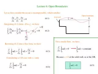
1. Lecture 6: Open Boundaries Let us first consider the ocean is incompressible, which satisfies Open boundary Solid wall (6.1)  Integrating (6.1) from –H to  , we have H (6.2) For a steady flow, we have Rewriting (6.2) into a flux form, we have (6.3) Because u= 0 at the solid wall, so at the OB, Considering a 2-D case with x-z only (6.5) (6.4)

2. OB N-3 N-2 N-1 N For an unsteady flow (6.4) If we could determine the flux at the OB, we should be able to calculate the temporal change of the surface elevation; Or in turn, if we know the temporal change of the sea level, we should be able to determine the flux at OB. Example (6.6) Differencing (6.6) using the central difference method for space, we get at OB There are no sufficient information to determine the current and surface elevation at OB!

3.  u  u  u  OB N-3 N-2 N-1 N If one uses the first order “backward” scheme for space, we could get You have the enough information to determine the current and surface elevation at OB, but works only when the wave propagates toward the OB from the interior! If one uses the staggered grid like Once the surface elevation at OB is determined, one could easily determine current at the velocity point closest to OB! QS.1: How could we determine the surface elevation at OB? For tidal forcing, we could specify it from the observational data, but for wind-driven circulation, we don’t know its value at OB QS.2: If we have to specify the OB value, what principal do we need to follow? 1) Mass conservation, 2) No reflection or minimizing reflection (regarding waves).

4. 1. Periodic OBC k = N k =1 If we know the wave length and also know the temporal change of the sea level (or current) at k =1 is the same as that at k = N, we cansimply the OBC to be Periodic condition QS: Could you give me some examples you could use this condition in the ocean modeling?

5. 2. Radiation OBCs (6.7) where c is the phase speed, and  can be either sea surface elevation or the cross OB velocity. The positive sign is used for the right open boundary at (x = W) and negative sign is used for the left open boundary at (x = 0) Choice 1: Clamped (CLP) (Beardsley and Haidvogel, 1981) (6.8) Consider a wave of unit amplitude travelling in the + x direction with frequency  and wavenumber k, where t = n∆t and x = j∆x The sum of the incident and reflected waves at OB equals to OB Incident wave (6.9) Reflected wave For CLP, 100% reflected!

6. Choice 2: Gradient (GRD) (6.10) Let us discuss the reflection rate of GRD, and the sum of the incident and reflected waves at OB is given as Applying it into (6.10) and considering the OB at x =0, we have (6.10)

7. Choice 3: Gravity-wave radiation: Explicit (GWE) The difference form of this condition is given as Using the same method shown in choices 1 and 2, we can obtain (6.11) It follows that the GWE is not free-reflected scheme.

8. Choice 4: Gravity-wave radiation: Implicit (GWI) The difference form of this condition is given as Using the same method shown in choices 1 and 2, we can obtain (6.12) Changing into the implicit scheme does not help to reduce the reflection!

9. Choice 5: Partially Clamped-Explicit (PCE) The difference form of this condition is given as Using the same method shown in choices 1 and 2, we can obtain (6.12) One could adjust to reduce the reflection.

10. Choice 6: Partially Clamped-Implicit (PCI) The difference form of this condition is given as Using the same method shown in choices 1 and 2, we can obtain (6.13) One could adjust to reduce the reflection.

11. Choice 7: Orlanski Radiation: Explicit (ORE) Assume that The reflection rate for ORE is (6.14)

12. Choice 8: Orlanski Radiation: Implicit (ORI) The finite-difference scheme, c and  are the same as ORE, except The reflection rate for ORI also is (6.14) Theoretically speaking, ORE and ORI are the best methods with no reflection. However, because many numerical errors are nonlinear coupled with momentum and tracer equations, ORE or ORI Does not guarantee no reflections all the time.

13. Sponge layer Add a sponge layer at the open boundary to dissipate the reflected energy. It is really a frictional layer which damps both incident and reflected waves. Sponge layer OBC Therefore, You can also different form of the friction, for example, exponentially function, etc. Note: the sponge layer tends to absorb all the waves into this layer, which includes both true incident waves plus numerical reflected waves. If the sponge coefficient is too big, it would destroy the numerical solution in the interior. Therefore, the sponge layer should only be used to improve the open boundary radiation boundary condition!

14. As GWE =0.5 Reflection rate approaches zero. In general, however, the reflection rate depends on the incident frequency and wavenumber as well as the numerical grid space and time step. For GWE and GWI, the minimum reflection is along the line of GWI =0.5 When the phase speed of the incident wave is equal to the assumed phase speed of the OBC, the reflection is minimum. GWE =1.0 There is always some reflection on the phase line, which is due to the numerical dispersion.

15. W = 160 km Numerical experiments: Barotropic relaxation ∆x and ∆y = 10 km L = 105 km where jm is the grid point in the middle of the numerical domain and y = m ∆y CLP PCI ORI Total energy plot: GRD Dashed line: the solution with perfectly transparent cross-shelf boundaries; Solid line: the numerical solution. MOI GWI SPO

16. Sea level

17. Friction roles in reducing the rms errors

18. Consider the wind stress Solution is This suggests an adjustment time of h/r for u to reach a steady state. With an assumption of the geostrophic balance in the alongshelf directon:

20. Consider a cross-shelf wind case with True solution: Along the infinite long coast, the response consists of oscillations due to gravity waves which radiate away from the coast leaving a steady state setup of sea surface elevation at the coast. What do you find from the right side figures?