Download
1 / 49
490 likes | 594 Views
Presentation on the measurement of gamma from Bs→DsK decay, including theoretical background, experimental status, and analysis strategies.

E N D
LHCb-ANA-2011-062 Approval Presentation, 17.08.11
Motivation for Measurement • The final state Ds-K+ is accessible by both Bs and Bs: • Both diagrams are similar in magnitude, hence large interference between them is possible. • Using flavour tagging, we can measure four decay rates • Bs or Bs to Ds+K- or Ds-K+ • From these rates, γ can be extracted in an unambiguous and theoretically clean way. • A review of the γextraction can be found in e.g. LHCb note 2007-041.
Branching Ratio Strategy • A reliable extraction of γ requires a considerable amount of data • Aim is to present first γ measurement from Bs→DsK at Moriond 2012. • First step towards measuring γ is to observe Bs→DsK in our data, and measure its branching ratio (BR) relative to Bs→Dsπ. • Most systematics cancel in the ratio • Main differences between the modes are the bachelor PID requirements and the smaller Bs→DsK yield. • Analysis strategy for the relative BR measurement follows that used for the hadronic fd/fs measurement from 2010 data. • Independently, the hadronic and semileptonic fd/fs measurements from 2010 data can be combined to extract BR(Bs→Dsπ). This is then used to measure BR(Bs→DsK) absolutely.
Current Experimental Status: DsK • PDG value is BR(Bs→DsK) = (3.0 ± 0.7)*10-4(23% relative error) • Calculated by rescaling Belle(*) measurement: BR(Bs→DsK)= (2.4 +1.2/-1.0(stat)± 0.3(syst) ± 0.3(fs) )*10-4. This uses 7±3 signal events. • In addition, CDF(**) measures BR(Bs→DsK)/BR(Bs→Dsπ) = 0.097 ± 0.018 ± 0.009 with ~100 DsK candidates, using a combined mass-PID fit. Bs→DsK Belle Bs→Dsπ CDF (*) PRL 102 021801 (**) PRL 103 191802
Current Experimental Status: Dsπ • BR(Bs→Dsπ) = (3.2 ± 0.5)*10-3(16% relative error), from combining • Belle(*): (3.67 ± 0.34(stat)± 0.43(syst) ± 0.49(fs) )*10-3 with 160 events • CDF(**) : (3.03 ±0.21(stat)± 0.45(syst) ± 0.46(fd/fs) )*10-4with 500 events Belle CDF (*) PRL 102 021801 (**) PRL 98 061802, rescaled to new BR(Bd→Dπ)
What about LHCb? • Today we are requesting approval of preliminary results for BR(Bs→DsK)/BR(Bs→Dsπ), BR(Bs→Dsπ) and BR(Bs→DsK). • We plan to write a paper in the very near future. • Plots for approval are marked with For Approval
Data Sample and Trigger/Stripping • The analysis uses ~336pb-1 of 2011 data. • Trigger requirements are • L0: Hadron TOS or Global TIS • HLT: HLT1Track and HLT2 Topo BBDT TOS (2,3 or 4 body) • Stripping lines from B2DX module (with D2hhh) • No PID is used, to allow inclusive selection of all the relevant modes • Relative efficiency of reconstruction, trigger and stripping is checked on MC that has been reprocessed with a 2011 TCK (0x006d0032) • Results on later slides
Offline Selection: BDTG • For the 2010 fd/fs analysis, TMVA was used to check the performance of different provide classifiers as an offline selection, using kinematic and geometrical variables • Role of the MVA is to minimise combinatorics (not physics backgrounds) • The best performing MVA was the Boosted Decision Tree with Gradient boosting (BDTG). • In the current analysis, the 2010 BDTG is retained, but optimal cut is re-evaluated • Optimal working point need not be the same, as the trigger has changed • Re-optimisation for 2011 is performed using 10% of the Bs→Dsπ data (uniformly distributed in time)
BDTG (Re-)Optimisation • Figure of merit is • Here, B refers to combinatoric bkg only, and 1/14 is the expected Cabibbo suppression factor between Bs→Dsπ and Bs→DsK. • Choose start of significance plateau (BDTG>0.1) as our working point. • This cut loses 6% of signal, for a background reduction of 45%.
PID Calibration • Correctly calibrating the PID cut efficiencies is crucial for this analysis. • Extensive use is made of the tools developed by the RICH group. • The D* (for K and π) and Λ (for proton) calibration samples are binned in momentum and pT, and the resulting efficiency map is used to weight signal events. • Magnet Up and Magnet Down data are calibrated separately • PID performance is not constant in time, as RICH calibration needs to be propagated to the more recent data • Separation between K and πis poor above 100GeV, hence apply a cut of p<100GeV on the bachelor. K eff π misID Example: DLL(K- π)>5 (1D binning for visualisation)
PID Cuts: D Daughters • For the moment, only the Ds→KKπ mode is considered • Other modes could be added in the future • To obtain clean samples of Bs→Dsh, PID cuts need to be applied to the D daughters to suppress Bd→D+h and Λb→ Λch. • Hence on the Ds+→ K-K+π+ candidate we require: • DLL(K- π) > 0 for the K- and DLL(K- π) < 5 for the π+ (to suppress combinatorics) • DLL(K- π) > 5 for the K+ (to suppress D+ →K-π+π+) • DLL(p-K) < 0 for the K+ (to suppress Λc+ →K- p π+) • K+ failing DLL(p-K) < 0 are retained if Kpπ mass is outside the Λc mass window • Applying these cuts and a mass window of [1944,1990]MeV gives: • Efficiency of 78% for Bs→Dsπ (using momentum distributions from MC), • MisID of 1.2% for Bd→D+π(using momentum distributions from data), • MisID of 1.7% for Λb→ Λcπ (using momentum distributions from MC).
Bs→Dsπ Purity after PID Cuts • After these cuts, the Bs→Dsπ peak is rather pure
PID Cuts: Bachelor • For the Dsπ fit, a cut of DLL(K-π)<0 is applied, to eliminate any residual contamination from DsK. • A hard cut of DLL(K-π)>5 is applied before doing the DsK fit, to suppress the favoured Dsπ mode. • As a cross-check, DsK fit is also done with a loose cut of DLL(K-π)>0, and a very tight cut of DLL(K-π)>10. • The efficiencies of these cuts, applied after the p<100GeV cut, are:
Efficiency Ratios from MC • Ratio of generator level efficiencies is found to be 1.027±0.010. Until the reasons for this are understood, the 1.027 is used as a correction factor, and a systematic of 2.7% is applied. • Ratio of efficiencies for reconstruction, trigger, BDT cut and upper momentum cut on the bachelor is 1.03±0.01. This correction factor is applied, and the associated systematic is conservatively set to 3%.
Signal Lineshapes • The B mass uses the D(s) mass constraint (improves resolution). • Different shapes are tested on the MC signal samples. • Deafult shape is double Crystal Ball, with common mean & sigma • Radiative tail is smaller for modes with bachelor K than bachelor π. Bs→Dsπ Bs→DsK
MisID Background Shapes • The physics bkgs to the different modes often involve misidentified hadrons. So getting the misID’d mass shapes correct is important. • Example: the shape for Dsπ bkg to DsK is obtained as follows: • Firstly, a clean sample of Dsπ is extracted from the Dsh data by applying DLL(K-π)<0 on the bachelor • This cut biases the bachelor momentum, however the original momentum distribution can be recovered from the whole Dsh sample • This works because the Dsπ and DsKbachelor momenta are very similar • Then the mass is recomputed under the DsK hypothesis • Next, the shape is weighted according to the momentum spectrum of the misidentified bachelors • This from the original momentum distribution and the misID rate as a function of momentum
MisID Background Shapes • The shape for Dπ bkg to Dsπ is obtained in a similar way, changing D daughter mass hypothesis instead of the bachelor. • The shape for the DKbkg to DsK should be the same as the Dπ bkg to Dsπ. • The shapes for Dsπ and Dπ under the DsK are sufficiently similar that in the fit only the Dsπ shape is used Under the DsK mass hypothesis
An Incidental Discovery… • A bump was seen in the DsKfit at around 5500MeV, that was not described by the misidentified Dsπ shape. • The bump was investigated, and it turned out to be Λb→Dsp! A peak is also seen at lower mass, compatible with Λb→Ds*p • A peak is seen at the Λb mass after switching to the Dsp mass hypothesis, applying extremely tight PID cuts (DLL(p-π)>10 and DLL(p-K)>15) on the bachelor, and tightening the BDT cut. • In the future a measurement will be made of the BR of this mode, but for now…
Λb→Ds(*)p ShapeUnder DsK • Cutting on DLL(p-K) would lose too much signal, so we must live with this background, and model its shape. • The shape is taken from simulated events, after reweighting for the efficiency of the DLL(K-π)>5 cut as a function of momentum. • The Λb→Ds*p shape is obtained by shifting the Λb→Dsp shape down by 200MeV. As a baseline, the relative amount of Λb→Dsp and Λb→Ds*p is assumed to be the same. • The amount of Λb→Dsp in the DsK fit is estimated by taking the 24 events from the previous slide, and correcting for the efficiency of the tight PID cuts and the BDTG cut. • This gives an expectation of ~150 events (Λb→Dsp + Λb→Ds*p) Λb→Dsp plus Λb→Ds*p
Partially Reconstructed (and other) Bkgs • For partially reconstructed physics bkgs, the shapes are taken from MC, with data-driven momentum reweighting applied where a misidentification is involved. PDFs are made using RooKeysPDF. • One final type of physics background needs to be considered: charmless modes such as Bs→K*KK • These can appear if no cut is applied on the flight distance of the D from the B vertex • They can peak under the signal • To remove such backgrounds, a soft cut of FDχ2(D from B) > 2 is applied. This will have the same efficiency for Bs→Dsπ and Bs→Dsπ, so will not affect the ratio of BR’s.
Combinatoric Background Shape • The slope of the combinatoric background can floated in the Dsπ fit. • However it must be fixed in the DsKfit, due to the low statistics and the presence of the misidentified Bs→Dsπ in the right-hand sideband. • Fitting to wrong-sign (same-sign D and bachelor) events passing the DsK selection and PID cuts, the slope is compatible with being flat. • As a cross-check, the wrong-sign events passing the Dsπ selection are also fitted, and the slope agrees well with that found in the Dsπ signal fit. DsK wrong-sign
Splitting by Magnet Polarity • Since the PID efficiencies vary slightly between MagUp and MagDown, the misID background shapes change. • In addition, the signal mean is found to shift by ~1MeV between MagUp and MagDown. • So we split the data by polarity, and fit the two subsamples independently. • About 55% (45%) of the data is MagDown (MagUp). • In the following slides, the MagDown fit is on the left, and the MagUp on the right.
Recipe for Dπ Fit • This fit is needed to estimate the amount of background Dπ to Dsπ, and to check the mean and sigma of the signal shape with high statistics. • The tails of the signal mass shape are fixed from the MC fit, but the mean and sigma are floated • Mean and sigma are allowed to be different for MagUp and MagDown • The yields of all components are left free. • The slope of the combinatoric background is also floated in the fit.
Recipe for Dsπ Fit • The expected number of misID Bd→Dπ is calculated using the fitted Dπ yield, a mass window factor (from MC), and misID from the PID calibration tools. • It is constrained to be within 10% of this estimate • The misID Bd→Dπ shape is also reweighted to take misID curve vs momentum into account. • The signal width is fixed to that found in the Bd→Dπ fit, scaled by the ratio of widths for Bs→Dsπ and Bd→Dπ in the MC • Signal mean and comb background slope are floating. • A Λb→ Λcπcomponent was allowed in the fit, but got fitted to zero. • Some Bd→Dsπ can also be seen • re-use Bs→Dsπ mass shape, and constrain yield to {known BR ratio*fd/fs} = 1/35 relative to Bs→Dsπ yield.
Fits: Dsπ with PIDK<0 For Approval For Approval
Recipe for DsK Fits • The amount of misID Bs→Dsπ background is floated • Provides x-check on misID rate estimate • Any Bd→Dπshould be taken care of by the Bs→Dsπ shape • Treatment of signal shape is the same as for Bs→Dsπ • Comb background slope is fixed to be flat (from wrong-sign) • Amount of Bd→DKisconstrained from the Bd→Dπ under Dsπ, using the Bd→DK/Bd→DπBR ratio • Relative yields of PartReco backgrounds are constrained using • Relative reconstruction efficiencies (from MC) when e.g. a charged track or soft pion/photon is missed • Bs branching ratios from Bdbranching ratios, using SU(3) symmetry • The yields can ove by 33% from these estimates • TheBd→DsKyield is floated. The Bs→DsKand Bd→DsKshapes are the same. • Amount of Λb→Ds(*)p is constrained as detailed earlier.
Fits: DsK with PIDK>5 (default) For Approval For Approval
Fits: DsK with PIDK>10 (cross-check) For Approval For Approval
Fits: DsK with PIDK>0 (cross-check) For Approval For Approval
Remark on Bd→DsK • While this component is clearly visible in the DsK fits, the amount of background underneath it makes a reliable fit to its yield very difficult, at least with the current dataset. • Hence we cannot make a competitive measurement of its BR (error in PDG is ~13%).
Systematics Menu for BR Ratio • Ratio of trigger/stripping/(non-PID) selection efficiencies from MC • Fit model systematics will be evaluated using a large number of toy fits (as was done for fd/fs analysis). • But for the moment, we simply apply cross-checks on the data, and assign conservative systematics. • For the PID, take systematic on efficiency curves quoted by the RICH group, evaluated at our cut values • PID systematic can enter in three different ways: • Final PID efficiency correction to obtain BR(DsK)/BR(Dsπ) • Shape of misID bkgs after reweighting • Expected number of Dπ/K under Dsπ/K (constrained in the fit)
Systematics Budget for BR Ratio • The fit model systematic for DsKis the most involved part of the systematics calculation. • The main contributions to this part are: • The slope of the combinatoric is fixed to half of the Dsπ slope. This reduces the signal yield by 3%. • The constraints on the partially reconstructed backgrounds are all varied by a factor of two. This changes the signal yield by ±4%. • Also, the ratio of the Λb→Ds*p component to the Λb→Dsp component was varied by a factor of two. The change to the signal yield is <0.5%.
Results: BR(Bs→DsK)/BR(Bs→Dsπ) • Averaging MagUp and MagDown, we get • N(DsK) = 406±26, N(Dsπ) = 6038±105 • εPID(DsK) = 83.4±0.2%, εPID(Dsπ) = 85.0±0.2% • εsel(Dsπ)/ εsel(DsK) = 0.945± 0.014 • We obtain
Extraction of BR(Bs→Dsπ) • Basically we turn the 2010 fd/fs combination on its head, by combining the ratio of yields of Bs→Dsπ and Bd→Dπ from the hadronic analysis, and the fd/fs value from the semileptonic analysis Input: Output:
Results: BR(Bs→DsK) • Combining these two results, we obtain • This agrees with the Belle result, but is significantly below the CDF result.
Conclusions • Using 2010 data we measure • With 336pb-1 of 2011 data we measure • These are combined to yield • These are all World’s Best measurements. • Last but not least, we would like to thank our referees, StefaniaVecchi and StephaneMonteil, for their quick work which has been very helpful in improving our analysis!
Extracting γ from DsK Strong phase difference
BDT Training (2010) • The MVA was trained for the fd/fs analysis using a small (2pb-1) subsample of the 2010 data • Several MVAs were tried, the Boosted Decision Tree with Gradient boosting (BDTG) was found to have the best performance
CDF Measurement PID variable (uses de/dx)
PID Efficiencies from Calib Tools These are for the bachelor momentum spectrum, after the p<100GeV has been applied.
Example of PartReco Bkg Shape for Bd→D*-π+ from 2010 MC, under pion (left) and kaon (right) mass hypothesis for the bachelor
Comparison to Theoretical Expectation • As a side-product of the 2010 fd/fsanalysis, we measured: • Whereas we now measure : • Bd→DKHas only one tree diagram, while the Bs→DsKhas two • So our result suggests that the two different tree diagrams contributing to the DsK final state interfere destructively