Lecture 4
330 likes | 698 Views
Lecture 4. Equilibrium and noequilibrium processes. Adiabatic, isotermic, isobaric and isochoric processes. Connection between statistical and thermodynamic quantities. Helmholtz free energy F , Enthalpy H and Gibbs Free Energy G . Thermodynamic potentials and Heat capacity.

Lecture 4
E N D
Presentation Transcript
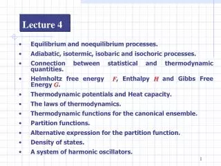
Lecture 4 • Equilibrium and noequilibrium processes. • Adiabatic, isotermic, isobaric and isochoric processes. • Connection between statistical and thermodynamic quantities. • Helmholtz free energy F, Enthalpy H and Gibbs Free Energy G. • Thermodynamic potentials and Heat capacity. • The laws of thermodynamics. • Thermodynamic functions for the canonical ensemble. • Partition functions. • Alternative expression for the partition function. • Density of states. • A system of harmonic oscillators.
Equilibrium and noequilibrium process The typical example of nonreversible( in statistical sense) process is the relaxation process. The process is reversible if during every it’s moment the system is in equilibrium state and the process can go any direction. The reversible processes are usually connected with some variations of external conditions and the energy of the system. The variations have to be so slow that the system can reach equilibrium. Very slow process can be defined as quasystatic. The meanings «slow» depends on process time and have to be compared with the relaxation time. Adiabatic processes can be defined as the processes at the constant material and temperature conditions. Isothermal, isobar andisochoricprocesses are going at a constant temperature, pressure and volume respectively
Connection between Statistical and Thermodynamic Quantities We have seen that for a system in equilibrium =(E,x,Ni), where E is the energy; x denote the set of external parameters describing the system; and the Niare the numbers of molecules of the several chemical species present. If the conditions are changed slightly, but reversibly in such a way that the resulting system is also in equilibrium, we have (4.1)
We may write this result as (4.2) Let us first consider a simple example with the number of particles fixed and the volume as the only external parameter; (4.3) Then from (4.2) (4.4) We see that the change in internal energy consists from two parts. The term d represents the change in internal energy when the external parameters are kept constant. This is just what is meant by heat. Thus
(4.5) is the quantity of heat added to the system in a reversible process. The symbol D is used instead of d because DQ is not an exact differential-that is, Q is not a state function. The term - dV is the change in internal energy caused by the change in external parameters; this is what we mean by mechanical work, and (4.6) is the work done on the system in the volume change dV. By elementary mechanics the work done must be given by -pdV. Therefore (4.7)
where p is the pressure. We see that (4.2) is equivalent to the equation (4.8) which is the First Law of Thermodynamics. The statement that dS=DQ/Tis a perfect (exact) differential in a reversible process is a statement of the Second Law of Thermodynamics. That is, DQ/T is a differential of state function, entirely defined by the state of the system. Now from (4.5) we know that
Specific Heat (4.9) is a perfect differential, as is a state function. We note that both 1/T and 1/ are integrating factors for DQ. As we know that =kT, thus (4.10) as the connection between the usual thermodynamic entropy S and the entropy as we prefer to define it for use in statistical mechanics. The specific heat at constant volume Cv, and the one at constant pressure, Cp, would be given by
We defined E as a function of and V. Other quantities of interest are then obtained from E: (4.11) whence (4.12) and (4.13) The independent variablesand V are often quite inconvenient and it is more convenient to work with , p or , V for example.
To do this we introduce auxiliary functions called thermodynamic potentials:F, H, G. Helmholtz Free Energy F F(V, ) is defined as (4.14) Now (4.15) From (4.15) (4.16) and (4.17)
Therefore if V, are the independent variables it is natural to introduce F, from which p, are readily calculated Enthalpy H H(,p) is defined by (4.18) Now (4.19) whence (4.20) and (4.21)
Gibbs Free EnergyG G(,p) is defined by (4.22) Now (4.23) whence (4.24) and (4.25)
The Helmholtz free energy of a body has the property that the work done on the body in a reversible process at constant temperature is the change of its Helmholtz free energy. This easily shown: in a reversible process (4.26) Note that -dF is the maximum work, which can be, done by the system in a change at constant temperature. In the case of one component system with the volume as only one external parameter we can write the main thermodynamic equation for quasi-static processes (4.27)
Energy E(,V,N) dE=-pdV+dN Entropy (E,V,N) d=dE+pdV-dN Enthalpy H(,p,N)=E+pV dH=d+Vdp+dN Helmholtz Free Energy F(,V,N)=E- dF=-d-pdV+dN GibbsThermodynamic Potential G(,p,N)=F+pV=N dG=-d+Vdp+dN Great potential (,V,)=F-N=-pV d=-d-pdV-Nd Thermodynamic potentials
Recapitulation of thermodynamic laws -postulated the existence of equilibrium states. All parts of closed equilibrium system are in the state of internal equilibrium and heat equilibrium between each other, that means one general characteristic from all subsystems is taking place (temperature principle). Zero law the law of energy continuity. The energy can be transformed to the system by the heat. It impossible to make any work without the energy. (The perpetual mobile of the 1st order is impossible). First law-
the entropy of the close system is increasing. It can be defined also through the Clausius principle: as the irreversible process of the transforming the heat from the hot body to the cold one. Second law- As the principle of Kelvin (Tomson) the second law read: It is impossible to build the cycle machine that can work by absorption of the heat from the thermostat with any other changes in the system (the perpetual mobile of the 2nd order can not be created). (Nernst-Plank heat theorem) - the entropy of the system is going to zero if the absolute temperature is also tends to zero. Third Law -
Thermodynamic Functions for the Canonical Ensemble Let us define the entropy of the canonical ensemble with mean energy <E> as being equal to the entropy of a microcanonical ensemble with energy <E>. This corresponds to the thermodynamic situation because in thermodynamics the entropy is fixed by the energy independently of whether the system is isolated or in contact with a heat bath. The entropy for the microcanonical ensemble is equal to lnwhere is the volume of phase space corresponding to energies between E0 and E0+E. As we have seen, the precise value of E isunimportant and we may choose it equal to the range of reasonable probable values of the energy in the canonical ensemble.
Let us first write in terms of E. If (E)denotes the volume of phase space corresponding to energies less thanE we have (4.28) We now estimate E, the range of reasonable probable values for the canonical ensemble. Let p(E)dEbe the canonical ensemble probability that the system will have energy in the range dE atE. Then, (4.29) where (E) is the occupancy probability of a unit volume of phase space at energy E.p(E) is distributed according to the Gauss distribution. The function is normalized and this means that we may estimate the breadth E of the distribution peak by
(4.30) i.e., by (4.31) Substituting the E given by this equation in the expression for , we obtain, using (3.39) (4.32) so that (4.33) We have
(4.34) But we recall the Helmoholtz free energyFE-, whence (4.35) and (4.36) We have further, by the normalization of (4.37) and (4.38)
The partition function If we define thepartition function as (4.39) (classical) (quantum) (4.40) we have (4.41) The other thermodynamic functions can be calculated from the partition function, using thermodynamic potentials.
Alternative expression for the partition function. Density of states. In most physical cases the energy levels accessible to a system are degenerate, i.e. one has a group of states, grin number, all belonging to the same energy value Er . In such a case it would be more appropriate to write the partition function (4.42) the corresponding expression for Pr , the probability that the system be in any of the states with energy Er , would be
(4.43) Clearly, the gr states with a common energy Erare all equally likely to occur. As a result the probability of a system having energy Erbecomes directly proportional to the multiplicity gr of this level; gr thus plays the role of "weight factor" for the level Er. The actual probability is then determined by both the weight factor gr and the Boltzmann factorexp(-Er/kT) of the level, as we indeed have in (4.43). Now in view of the largess of the number of particles constituting a given system and the largess of the volume to which these particles are confined, the consecutive energy values Erof the system must be extremely close to one another.
Accordingly, there lie, within any reasonable interval of energy (E,E+dE), a very large number of energy levels. One may then regard Eas a continues variable and write P(E)dE for the probability that the given system, as a member of the canonical ensemble, may have its energy in the specified range. Clearly, the product of the relevant single-state probability and the number of energy states lying in the specified range will give this. Denoting the latter by g(E)dE, where g(E) stands for the density of states of the system around the energy value E, we have (4.44)
which on normalization becomes (4.45) The denominator is clearly another expression for the partition function of the system: (4.46) The expression for <f> any average value of physical quantity f may be written in this case as
The integral is, of course convergent over the positive half plane of (because g(E)0 for allE and for all >0). (4.47) Let us consider the relation (4.46) If we regard =1/kT as a complex variable, then the partition function Z()is just Laplace transform of the density of statesg(E). We can, therefore, write g(E) as the inverse Laplace transform of Z()
(4.48) the path of integration runs parallel to, and to the right of, the imaginary axis, i.e. along the straight line Re = >0.
A system of harmonic oscillators We shall now study, as an example, a system of N, practically independent, harmonic oscillators. We start with the specialized situation when the oscillators can be treated classically. The Hamiltonian of any one of them (assumed to be one-dimensional) may then be written as (4.49) of course, the index i will run from 1 to N. For the single-oscillator partition function, we readily obtain (4.50)
where The partition function of the N-oscillator system would then be (4.51) The Helmholtz free energy of the system is now given by (4.52) whence we obtain for other thermodynamic quantities (4.53) (4.54) (4.55) (4.56) (4.57)
We note that the mean energy per oscillator is in complete accord with the equipartition theorem, namely 2 , for E we have here two independent quadratic terms in the single oscillator Hamiltonian. We may determine the density of states, g(E),of this system from the expression (4.51) for its partition function. We have, in view of (4.48), ('>0), that is (4.58)
To test this correctness, we may calculate the entropy of the system with the help of this formula. Taking N>>1 and making use the Stirling approximation, we get (4.59) which yields for the temperature of the system (4.60) Eliminating E between these two relations, we obtain precisely our earlier result for the functions S(N,T). This indeed assure us of the inner consistency of our approach: more so, it gives us confidence to accept (4.58) as the correct expression for the density of states of this system.
We now take up the quantum-mechanical situation, according to which the energy eigenvalues of a one-dimensional harmonic oscillator are given by (4.61) n=0,1,2,... Accordingly, we have for the single-oscillator partition function (4.62) The N-oscillator partition function is then given by (4.63)
For the Helmholtz free energy of the system, we have (4.64) whence we obtain for other thermodynamic quantities (4.65) (4.66) (4.67) (4.68)
