Download
1 / 28
280 likes | 382 Views
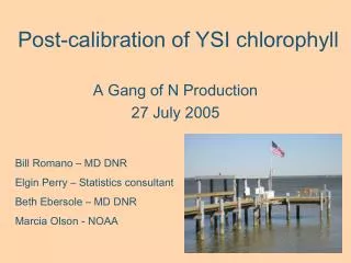
Post-Calibration of Fluorescence Data from Continuous Monitors (To adjust or not to adjust, and if so, how?). A “Gang of N” Production Elgin Perry - Statistics Consultant Marcia Olson - NOAA/CBP Beth Ebersole - MD DNR Bill Romano - MD DNR.

E N D
Post-Calibration of Fluorescence Data from Continuous Monitors (To adjust or not to adjust, and if so, how?) A “Gang of N” Production Elgin Perry - Statistics Consultant Marcia Olson - NOAA/CBP Beth Ebersole - MD DNR Bill Romano - MD DNR Presented to the Tidal Monitoring and Analysis Workgroup on 3 December 2003
Diel cycle Tidal cycle
log(x/y)=log x - log y LNRAT = LNCHL_F – LNCHL_A
Model Evaluated Log ratio as a function of: • Season • Sonde deployed • Light • Turbidity
At higher light levels, extractive samples exceed fluorescence data?
Fluorescence exceeds extractive at all light levels, so no light effect.
Fluorescence exceeds extractive under all light levels, so no light effect.
Chlorophyll Adjustment Methods • Regression method – CF(adj) = ß0 + ß1CF (Model CS = CF) • Multiple regression – CF(adj) = ß0 + ß1CF + ß2Turb (Model CS = CF, Turbidity) • Ratio method – CF(adj) = CF x (CS/CF) • Subtract “background fluorescence”
Linear Regression Assumptions • Y is linearly related to X • Expected value of the error term is zero • Constant variance in the error terms, which are uncorrelated • Independent variable(s) is measured without error • Independent variables are not linearly related
Conclusions • Stop collecting data • Full speed ahead (one size fits all) • Test various models and select one that minimizes root mean square error on a per station basis • Hire an expert to assess covariate measurement error problem • Log transform for correction and then back transform