Understanding Random Variables and Performance Estimation in Networking
This document explores the significance of modeling and estimating performance parameters in networking, particularly through the use of random variables. It covers essential traffic characteristics such as throughput, delay, and variability, alongside the importance of probability in understanding network protocols. Key concepts include probability distribution functions, moments, and Bayes' theorem, providing a foundation for examining traffic estimations, resource allocation, and performance analysis. This information is crucial for optimizing network routing and resource management.


Understanding Random Variables and Performance Estimation in Networking
E N D
Presentation Transcript
Random Variables Dr. Abdulaziz Almulhem
Preliminary • An important design issue of networking is the ability to model and estimate performance parameters • For example, estimate future traffic volumes and characteristics 2
Why do we need such estimates? • To study the effect of routing protocols • To estimate resources needed by reservation protocols • To study queuing discipline • To identify buffer sizes needed 3
Preliminary • Parameters used in characterizing data traffic: • Throughput characteristics: • Average rate: the load sustained by the source over a time period (resource allocation) • Peak rate: the max. load a source can generate (buffering might be needed for smoothing) • Variability: burstiness of a source 4
Preliminary • Delay characteristics: • Transfer delay: delay from source to destination • Delay variation (jitter): variation in transfer delay (impacts real-time applications) 5
What’s next? • We need to know little about probability • Random variables • What are they? • Their properties • Examples 6
Probability Premier • Probability P(A) of an event A is a number that corresponds to the likelihood that the event A will occur Sample Space (space of events) B A 0 1 P(A) P(B) 7
Definitions & observations • 0 P(A) 1 • P(Ai) = 1; Ai is an event in the sample space • P(A)= Na/N; • Na= number of outcomes in which A occurred (frequency) • N= total number of possible outcome 8
Definitions & observations • If two events A & B are mutually exclusive (independent) then: • Prob (A or B is to occur) =P(A) + P(B) • Prob (A and B to occur) =P(A) * P(B) • EX. Out of 2 apples and 3 oranges in a basket, what is the prob. of having 2 oranges when I need to grab three items from the basket? 9
Definitions & observations • The conditional prob. of an event A assuming the event B has occurred P(A|B) is (A & B are not independent): • P(A|B)=P(AB)/P(B) • If A & B are independent: • P(A|B)=P(A) & P(A|B)=P(B) 10
Baye’s Theorem • Given the set of mutual exclusive events E1, …, En • Ei covers an arbitrary event A • P(A)=in=1 P(A|Ei)P(Ei)=? Then P(Ei|A)=P(A|Ei)P(Ei)/P(A) E2 E1 A E3 11
Example Sender Receiver Given, S0 = event of sending 0 S1 = event of sending 1 R0 = event of receiving 0 R1 = event of receiving 1 P(S0) = p P(S1) = 1-p Also the received data (bits) can be observed P(R0|S1) = pa & P(R1|S0) = pb Physical Medium Network 0 0 Error 1 1 12
Example • Now to calculate the conditional probability of an error • That is a one was sent given that a zero is received P(S1|R0)= P(R0|S1) P(S1) / P(R0) Where P(R0) = P(R0|S0) P(S0) + P(R0|S1) P(S1) P(S1|R0)=pa p / [pa p+(1-pb)(1-p)] 13
Random Variables • RV is simply a numerical description of the outcome of a random experiment. • Examples: • Arriving customers at a given time • Tossing a coin • Packets in a switch at a given time • Etc. • We describe RV with distribution functions. 14
Cumulative distribution function (CDF) • CDF for an RV denoted FX(x) is defined as the probability that RV is less than or equal to x: FX(x) = p(X x) • F(-)=0; F()=1; 0F(x) 1 • F(x1) F(x2) when x1 x2 • p(x1 X x2) = F(x2) - F(x1) 15
Probability distribution function (pdf) • It is the derivative of CDF fX(x) = d FX(x) / dx 16
Moments • To completely characterize a RV, it is sufficient to know its pdf. • It is practical to describe some key aspects or few numbers of the pdf rather than specifying the entire pdf. • This is called moments or statistical avergares • Evaluated using the mathematical expectation 17
Mathematical expectation • The expected or mean value of an RV • Expectation is a linear operation 18
Moments • The mth-order moment of FX(x) is • Zero order =1 • First order is mean (previous slide) • Second is the mean-squared value 19
Moments (cont.) • Second moment is the variance and denoted by • Standard deviation is square root of variance and it measures the speard of observed values of the RV around its mean 20
Moments (cont.) • Third moment describes the skewness and characterizes the degree of asymmetry of the distribution around its mean. • It is a dimensionless quantity. • When zero distribution is symmetric • +ve leans towards the right; -ve leans towards the left 21
Moments (cont.) • Fourth moments defines kurtosis and measures the flatness or peakedness of a distribution about its mean. • It is dimensionless • It is relative to the normal distribution • More +ve means peaked distribution • More –ve means flatten distribution 22