Download
1 / 24
240 likes | 554 Views
Multi-scale modeling of the carotid artery. G. Rozema, A.E.P. Veldman, N.M. Maurits University of Groningen, University Medical Center Groningen The Netherlands. Area of interest. Atherosclerosis in the carotid arteries is a major cause of ischemic strokes!. distal. proximal.

E N D
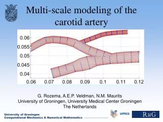
Multi-scale modeling of the carotid artery G. Rozema, A.E.P. Veldman, N.M. Maurits University of Groningen, University Medical Center Groningen The Netherlands
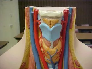
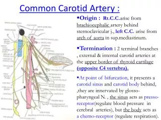
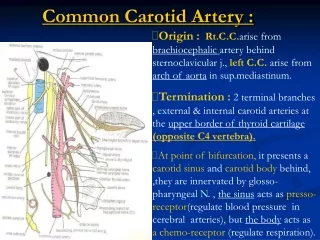
Area of interest Atherosclerosis in the carotid arteries is a major cause of ischemic strokes! distal proximal ACI: internal carotid artery ACE: external carotid artery ACC: common carotid artery
A model for the local blood flow in the region of interest: A model for the fluid dynamics: ComFlo A model for the wall dynamics A model for the global cardiovascular circulation outside the region of interest (better boundary conditions) Global Cardiovascular Circulation (electric network model) Multi-scale modeling of the carotid artery Several submodels of different length- and timescales Carotid bifurcation Fluid dynamics Wall dynamics
Finite-volume discretization of Navier-Stokes equations Cartesian Cut Cells method Domain covered with Cartesian grid Elastic wall moves freely through grid Discretization using apertures in cut cells Example: Continuity equation Conservation of mass: Computational fluid dynamics: ComFlo
The wall is covered with pointmasses (markers) The markers are connected with springs For each marker a momentum equation is applied x: the vector of marker positions Modeling the wall as a mass-spring system
Simple boundary conditions: Dynamic boundary conditions: Deriving boundary conditions from lumped parameter models, i.e. modeling the cardiovascular circulation as an electric network (ODE) Boundary conditions Outflow Outflow Inflow
Coupling the submodels Carotid bifurcation Weak coupling between fluid equations (PDE) and wall equations (ODE) Weak coupling between local and global hemodynamic submodels Future work: Numerical stability Fluid dynamics PDE wall motion pressure Wall dynamics ODE Boundary conditions Global Cardiovascular Circulation ODE
Global cardiovascular circulation model Carotid Bifurcation
Consider an elastic tube, with internal pressure P and volume V The linearized pressure-volume relation is given by Differentiate the PV relation and use conservation of mass to obtain C: Compliance of the tube Electric analog: Capacitor Q: Current, P: Voltage Qin Qout P, V P Qin Qout C Flow in tubes Compliance due to the elasticity of the wall P: Pressure in tube V: Volume of tube V0: Unstressed volume Qin: Inflow Qout: Outflow
Consider stationary Poiseuille flow (parabolic velocity profile) Conservation of momentum is given by: R: Resistance due to fluid viscosity Electric analog: Resistor Q: Current, P: Voltage Pin Q Pout Q Pin Pout R Flow in tubesResistance due to fluid viscosity Pin: Inflow pressure Pout: Outflow pressure Q: Volume flux
Consider inviscous potential flow (flat velocity profile) Conservation of momentum is given by (Newton’s law): L: Resistance due to inertia (mass) Electric analog: inductor Q: Current, P: Voltage L Pout Pin Q Flow in tubesResistance due to inertia Pin: Inflow pressure Pout: Outflow pressure Q: Volume flux Pin Q Pout
Linearized pressure-volume relation for elastic sphere Include heart action by making the compliance C time-dependent C(t): Time-dependent compliance of the ventricle Differentiate the time-dependent PV relation and use conservation of mass to obtain Qin P Qout C(t) 1/C’(t) -V0(t)/C(t) The ventricle modelElastic sphere with time-dependent compliance P: Pressure in sphere V: Volume of sphere V0: Unstressed volume P, V
Use the EDPVR and the ESPVR from the PV diagram of the left ventricle Assume a linear ESPVR and EDPVR with slopes Ees and Eed and unstressed volumes V0,es and V0,ed: Clinical applicationParameterization of the ventricle model: the PV diagram Ejection Relaxation Contraction Filling
Construct PV relations for intermediate times by moving between the ESPVR and EDPVR according to a driver function e(t) between 0 and 1: Example of a driver function e(t): Clinical applicationParameterization of the ventricle model: the driver function e(t)
Differentiate the time-dependent PV relation and use conservation of mass to obtain the ventricle model: with C(t): Time-dependent compliance, function of Ees and Eed M(t): Voltage generator, can be left out when assuming V0,es = V0,ed = 0 Qin P Qout C(t) 1/C’(t) M(t) Clinical applicationParameterization of the ventricle model: electric analog
Minimal electrical modelSimple ventricle model Peripheral resistance Carotid Artery Input resistance Ventricle model
Minimal electrical modelHeart valves modeled by diodes Carotid Artery
Minimal electrical modelInput/output compliance, resistance around ventricle Carotid Artery
Minimal electrical modelCompliance in peripheral element Carotid Artery
Minimal electrical modelParallel systemic loop, internal/external carotid peripheral elements Carotid Bifurcation
Structure of the model Red: Arterial compartments Blue: Venous compartments Green: Capillaries Carotid Bifurcation
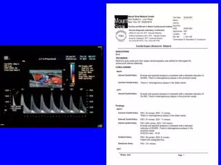
A simulation is performed to see if the model can capture global physiological flow properties: Parameter values are not yet realistic Simulation example Simulated flow rate for two cycles
Simulation example • Left ventricle simulation results show global correspondence to real data (Wiggers diagram) Aortic valve closes Aortic valve opens Pressure in left ventricle (solid) Pressure in aorta (dash) Volume in left ventricle
Parameterization of the electric network model (resistors, inductors, capacitors): linking the model to clinical measurements Coupling of the electric network model to the 3D carotid bifurcation model Multi-scale simulations for individual patients? Future work