Adaptive Multi-scale Modeling

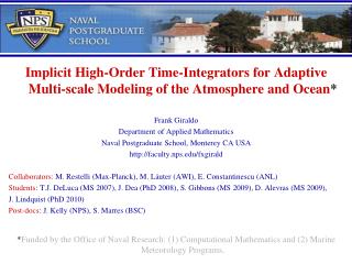
1. Implicit High-Order Time-Integrators for Adaptive Multi-scale Modeling of the Atmosphere and Ocean* Frank Giraldo Department of Applied Mathematics Naval Postgraduate School,Monterey CA USA http://faculty.nps.edu/fxgirald Collaborators: M. Restelli (Max-Planck), M. Läuter (AWI), E. Constantinescu (ANL) Students: T.J. DeLuca (MS 2007), J. Dea (PhD 2008), S. Gibbons (MS 2009), D. Alevras (MS 2009), J. Lindquist (PhD 2010) Post-docs: J. Kelly (NPS), S. Marres (BSC) *Funded by the Office of Naval Research: (1) Computational Mathematics and (2) Marine Meteorology Programs.

2. Adaptive Multi-scale Modeling • Multi-scale Modeling is an important research topic in all areas of computational mathematics and engineering (journals and conferences have emerged with this title). • Most GFD applications involve processes of varying spatial scales: think of a global NWP model trying to resolve simultaneously large-scale patterns and extreme events (such as hurricanes). For Ocean models think of simulating the propagation and run-up of storm surges. • Adaptive Methods (AM) are the natural choice for attacking these problems - the premise is to automate/adapt the resolution of the model to the underlying multi-scale physics of the problem. • In this talk, we will discuss some of the many issues facing the successful construction of AM for improving the solution of multi-scale problems in Computational Geophysical Fluid Dynamics.

3. Talk Summary • General Classification of Adaptive Methods (AM) • Standing Issues for Adaptive Methods • Time-Stepping Strategies • Time-Integration and Boundary Conditions • Sample Simulations • Closing Remarks

4. I. Adaptive Methods (AM)

5. General Classification of Adaptive Methods • R-refinement: The number of points remains constant for all time; however, the position of these points move (e.g., Prusa-Smolarkiewicz 2003) . • H-refinement: The number of grid points changes with time (e.g., Berger-Oliger 1984, Skamarock-Klemp 1993, Giraldo 1995, Behrens 1998, Blayo-Debreu 1999, Giraldo 2000, Hubbard-Nikiforakis 2003, Piggott et al. 2005, Jablonowski et al. 2005, St.Cyr-Jablonowski 2008, Weller-Weller 2008). • P-refinement: The number of grid points and their locations remain the same, the number of modes used to construct the solution changes. This is only possible with Galerkin methods. • CG Approach: can only be used with a set of modified hierarchical (modal) basis functions. • DG Approach: this idea can be naturally extended to DG methods. The application of limiters can be viewed in this light. • HP-refinement: Combining AMR (h-refinement) with limiters in a Godunov method (FV, DG) is currently the best strategy. However, AMR with DG (high-order FV) is not very common (e.g., Bernard, Chevaugeon, Legat, Deleersnijder, Remacle 2007). • Key Point: All these methods move points closer together so that “special” handling of the time-step must be considered.

6. Examples of Structured Grids Banded Hexahedral Telescoping

7. Examples of Unstructured Grids Icosahedral-Quads Adaptive (Courtesy of Jörn Behrens) Icosahedral Adaptive

8. II. Some Standing Issues for Adaptive Methods

9. Some Standing Issues for Adaptive Methods • Parallelization/Domain Decomposition: Modifying the data structures dynamically slows the computations. E.g., the domain decomposition needs to be a direct by-product of the adaptive mesh generator. A good first candidate for AM is statically adaptive grids where the grid is modified and held fixed for the entire simulation. This must work well before moving onto dynamically adaptive grids. • Coupling of Dynamics and Physics: Sub-grid scale parameterization is notoriously inconsistent meaning that changing the grid resolution changes the results. Also, the dynamics must use the “proper” approximations for the smallest scales. This means that both Atmospheric and Ocean codes should use the nonhydrostatic equations. This has direct effects on the time-integration strategies (IPAM 2010 Workshop) as faster waves (e.g., vertically propagating “acoustic” waves) must be considered in the choice of time-step.

10. Some Standing Issues for Adaptive Methods(Continued) • Error Indicators: This is the mechanism by which an adaptive mesh generator decides to coarsen or refine the mesh. The question we need to know a priori is what sorts of processes do we wish to track (error indicators try to equi-distribute the error in a global sense). The error indicator can do its job iff the spatial and temporary resolutions have high fidelity. This means that spatial, temporal, and boundary conditions should have a balanced order of accuracy. • Handling Time-stepping: By definition, multi-scale problems have processes occurring at all spatial scales that then require special treatment with respect to time in order to run efficient simulations (stiff and non-stiff parts). • For explicit methods, the time-step has to be small enough to maintain stability wrt to the fastest waves in the system and the smallest cells in the grid (subcycling). • For semi-implicit methods, one must still must adhere to the time-step stability of the nonlinear terms (Rossby waves). • There has been much work on constructing high-order spatial discretization methods but not as much effort has been spent on implicit time-integration. • High-accuracy yet efficient time-integrators can be obtained. These methods are easily modified to yield variable order in time with adaptive time-stepping.

11. III. Time-Stepping Strategies 1. Explicit Time-Integrators2. Semi-Implicit (IMEX) Time-Integrators3. Lagrangian Time-Integrators4. Fully-Implicit Time-Integrators

12. 1. Explicit Time-Integrators • Let’s write the governing equations as • SSP-RK(2,3,4) For k=1,…,K • SSP-BDF2 Which we write as or in general (Kth Order), more compactly, as

13. 2. Semi-Implicit (IMEX) Time-Integrators(Building an implicit method on top of an explicit one) • Let’s start with • Now, if we knew the linear operator L, then we could write • Discretizing by Kth order time-integrator yields Where and

14. 2. Semi-Implicit (IMEX) Time-Integrators(Constructing the Schur Complement) • The implicit problem that we have is: • Where the dims are: • For 2D Euler d=4, 3D d=5, etc. • For 2D Euler we solve a 16N2 system • For 2D SWE d=3, and solve a 9N2 • A better approach is to write out the system as follows (for 2D SWE): • Applying block LU decomposition: • Where the Schur Complement is: • And the dimensions are:

15. 2. Semi-Implicit (IMEX) Time-Integrators(Important Properties of Schur Complement) • The original system is: • The Schur Complement system is: • This system is clearly smaller than the original system (NxN instead of 3Nx3N for 2D SWE). • Equally important is that the Schur System is better conditioned than the original system. This means that fewer iterations are required by an iterative solver to reach convergence. • Key Point: A semi-implicit method should be more efficient than the most efficient explicit methods, but with the addition of the Schur Complement system, the gains are much bigger. Thus, whenever possible we must strive to find such a system. This is not always very easy.

16. 2. Semi-Implicit (IMEX) Time-Integrators (BDFK)(SWE: Linear Kelvin Wave) Performance Accuracy DG with N=10

17. IMEX BDFK Time-Integrators(Stability Regions) Explicit Implicit

18. 2. Semi-Implicit (IMEX) Time-Integrators(Which Methods offer a Schur Complement?) • The general belief is that a Schur Complement • can only be extracted from single-stage multi-step methods (e.g., LF, BDF, AB, etc.) • Cannot be extracted from multi-stage single-step methods (e.g., RK methods). • It turns out that it can be done as long as one can write the method in the IMEX form: • Additive Runge-Kutta Methods can be written in the Schur Complement form. This now extends the order of accuracy in time as well as the maximum time-step allowed for efficiency (big gains in the explicit part for increasing K).

19. 2. Semi-Implicit (IMEX) Time-Integrators(Additive RK Methods) • Starting with: • We can then write this in the IMEX form: • Discretizing by Kth order time-integrator yields For k=1,…,K Where and

20. Additive Runge-Kutta Time-Integrators(Stability Regions) ARK3 ARK3 RK3 BDF3 RK2 Implicit Explicit Analysis performed by E. Constantinescu (ANL)

21. 3. Lagrangian Implicit Time-Integrators(Building Lagrangian method on top of semi-implicit) • Let’s rewrite the governing equations as • Which, after introducing the Lagrangian derivative, allows us to write • Once again, we use L to write • Which, again, yields: • Where the variables depend on the time-integrator used (for either BDF or ARK as shown previously).

22. 4. Fully-Implicit Time-Integrators • Writing the governing equations as • We then discretize this implicitly using implicit methods (eg., BDFK, IRK) • Where the matrix problem is now • Which clearly requires a nonlinear implicit solution(eg., Newton-Krylov methods) • We write the problem as the functional: • And then solve the nonlinear problem:

23. IV. Time-Integration and Boundary Conditions

24. Implementing Boundary Conditions • For explicit time-integrators, implementing BCs is trivial (a posteriori). • For semi-implicit/implicit time-integrators, the BCs have to be incorporated into the time-integrator. • BCs can be generalized quite naturally via Lagrange multipliers as such: • Where “tau” satisfies all BCs including NFBC and NRBCs • We are currently extending high-order BCs into this formulation.

25. Balancing All Errors(N=K=J=4) Simulation performed by J. Lindquist (NPS) as part of his PhD Thesis

26. V. Sample Simulations

27. V. Simulations: Mesoscale Model

28. Convective Storm Simulation(500 x 200 meter resolution, N=10, K=2, J=10) Vapor Rain Clouds

29. Riemann Problem(Np=40,000 N=1, K=2, Lon=180, Lat=0) V Height U

30. Circular Dam Break(h-refinement, N=1, K=3, J=1) Ne=17,000 Ne=80,000 Ne=20,000

31. Circular Dam Break(hp-refinement, N=0/1, K=3, J=1) Ne=17,000 Ne=80,000 Ne=20,000

32. V. Simulations: Oceanic Shallow Water Model

33. Rossby Soliton Wave in a Channel(N=8, K=3, J=8) Ne=260 Ne=250

34. Rossby Soliton Wave in a Channel(Np=8113, Ne=250, N=8, K=2, J=8) y Grid x Free Surface Height

35. Propagation of the 2004 Indian Ocean Tsunami(Grid Dimensions: Np=66715, Ne=130444, N=1, K=2, J=1) y x Time evolution of the water surface height (grid data provided by J. Behrens, AWI, and data formatted by D. Alevras, NPS)

36. VI. Closing Remarks • There is no doubt that AM is the key to resolving multi-scale problems but the question we need to answer is: what goal are we trying to achieve? Should we expect to focus on more than one process. If so, under what conditions is this useful. E.g., tracking a hurricane within a global atmospheric model, or a storm surge in an ocean model. • Statically AM is definitely useful now in mesoscale atmospheric and ocean models and are already being used – but this can be exploited more than has been previously. • For NWP studies, the codes need to be “fast” in order to be used operationally. Can the construction of the new grids and corresponding data structures be sped-up to make it worthwhile to invest in adaptivity versus global high-resolution everywhere?

37. VI. Closing Remarks (continued) • There needs to be a significant investment in sub-grid scale parameterizations, we hear primarily about new dynamics with new grids but the reality is that the physics is mostly responsible for the quality of the results. • Time-Integrators that are able to handle accurately and efficiently the disparate spatial scales of a problem must be explored. Time-integration is a frontier that has also been overlooked especially by the GFD (spectral transforms) and high-order spatial discretization methods community (e.g., spectral elements); FV/DG communities have viewed space-time together (e.g., Godunov methods and RKDG). New classes of semi-implicit and fully-implicit time-integrators need to be explored along with their corresponding preconditioners and iterative solvers. The boundary conditions should also be taken into account as a part of the space-time domain. • Funding Agencies need to be made to understand that there is a potential pay-off if we invest in adaptivity. Currently, agencies do not see this need (at least not in the U.S.). ICON is the only modeling effort that I know of that has adaptivity as a prerequisite. This lack of funding/interest in AM exists in both Atmosphere and Ocean funding agencies. One possible fix is to invite funding agencies to workshops such as this one.