Geogg124 Terrestrial Ecosystem Modelling

1. Geogg124Terrestrial Ecosystem Modelling P. Lewis Professor of Remote Sensing UCL Geography & NERC NCEO

2. Aims of lecture • In this lecture, we will consider: • Land surface schemes • Global vegetation modelling • Production efficiency models • Phenology • Modelling Photosynthesis

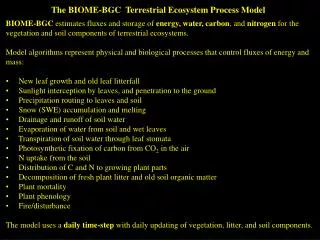
3. 1. Land surface schemes • LS schemes, implemented as LS models • LS component of climate / earth system models • Purpose: • Model energy and (carbon, water) fluxes at land-atmosphere interface

4. Main driver: energy • Rn=S↓(1−α)+L↓−L↑ • Rn = net radiation; S↓ = downwelling s/wave; α= albedo; L↓, L↑down/upwelling longwave • terms balance globally over the long term • But short term /spatial variations drive earth system

6. Balance by heat & chemical fluxes • Rn=H+λE+G+F • H = sensible heat flux; λE= latent heat flux; G = soil flux; F = chemical energy flux stored in photosynthesis • Latent heat – heat absorbed/released by change of state at constant T (eg liquid to vapour) • Sensible heat – causes solely change in T

8. Partitioning latent & sensible heat • Partitioning important as controls flux of water vapour to the atmosphere • Influence on cloudiness, rain • Hand λE are turbulent heat fluxes • Ts = surface T; Tr = ref. temp. above surface; ra = aerodynamic resistance; ρ = density of air; c.r = specific heat of air. e*(Ts) is saturated vapour pressure at Ts; er = vapour pressure at ref height; v = psychometric constant; rs = bulk surface resistance to transfer of water to air.

9. surface and aerodynamic resistances for water vapour flow

10. Roughness length depends on vegetation height Removal of vegetation can have feedback effect

11. Other fluxes • Turbulence also affects other fluxes e.g. CO2 • So we can relate internal and ambient CO2 to stomatal and aerodynamic resistance Approx.

12. Water balance • P=E−Rdrain−Rsurf−ΔS So we can relate evapotranspiration to runoff, change in soil water storage and water inputs (precip., snowmelt) P = water input; E = evapotransp.; Rdrain = slow drainage; Rsurf = surface runoff; ΔS = change in soil moisture storage

13. Land Surface Model • Models energy and water fluxes (++) at the land surface • provides an interface of these to atmospheric modelling. • Usually, this will be done for a set of grid cells, where inputs and outputs of each cell are considered separately • Lateral transport of water (e.g. snow, river)

14. Basic vegetation growth

15. Structure of most models similar

16. Some land surface schemes:Third generation LSMs • 1990s+ • Advance LSM by connecting leaf stomatal conductance and carbon assimilation • Farquhar et al. (1980) and Farquhar and von Caemmerer (1982) • Can dynamically model vegetation • Examine climate feedbacks

18. 1. Land surface schemes • Summary • outlined the main processes in land surface schemes and models and highlighted the interplay of radiation and water. • introduced some core concepts in vegetation processes • vegetation growth can be modelled as a potential amount of carbon assimilation that is then limited by factors such as water and nutrient availability as well as being reduced by pests, disease etc. • Looked at some features of 3rd generation LSMs • Include carbon

19. 2. Global vegetation modelling • Focus on linking measurements from Earth Observation and other sources with models of terrestrial carbon at regional and global scales. • motivation for models • to express current understanding of the controls on carbon dynamics as embedded in Earth System / Terrestrial Ecosystem models. • The role of observations is to test and constrain these models to enable: • (i) monitoring of terrestrial carbon dynamics; • (ii) improved prognostic models. • The main focus of the modelling and monitoring is on Net Primary Productivity (NPP).

20. Types of models • TEMs • Static vegetation representation • DGVMs • Dynamic vegetation • PEMs • Simplifications for ‘data driven’ model

21. Dynamic Global Vegetation Models

22. DGVMs • Main components: • establishment, • productivity and competition for resources, • resource allocation, • growth, • disturbance and mortality

23. DGVMs • Key features: • allows for prognostic and paleouse • geared towards modellingpotentialvegetation • anthropogenic influences e.g. changes in land use incorporated by forcing these effects • e.g. prescribing land cover/PFT

26. Dynamics, Establishment & Mortality

27. Plant Functional Types • Key simplification in DGVMs: PFTs • Group plant types by responses to resources and climate • Simplification allows global modelling • Limits number of parameters required • PFTs should: • represent the world’s most important plant types; • characterize them through their functional behavior; • provide complete, geographically representative coverage of the world’s land areas

29. Box et al. PFTs

30. Or Bonan et al., biome/climate rules

31. PFTs • Some issues: • Uncertainty from land cover • Variations in mappings to PFTs • Assume parameters describing functioning constant over PFT • New evidence from traits databases

33. Analysis of species/PFT in TRY http://try-db.org/pmwiki/index.php Kattge et al. (2011) GCB

35. How ‘good’ are these models? • Current benchmarking efforts • International Land Model Benchmarking – iLAMB • Previous (more limited) • Carbon-Land Model Intercomparison Project - C-LAMP • 2 models (CASA’, CN) • global carbon sinks for the 1990s differed by a factor of 2 • magnitude of net carbon uptake during the growing season in temperate and boreal forest ecosystems was under-estimated

36. How ‘good’ are these models? • Model intercomparisons (e.g. Sitch et al., 2008)

37. How ‘good’ are these models? • models estimates within range of current knowledge of C budgets and relatively close to the mean IPCC values. • The models in general agreement about the cumulative land uptake over the last 50 years. • Models simulated the correct sign of response to ENSO events but differed markedly in magnitude. • have similar response of productivity to elevated atmospheric CO2 in agreement with field observations • The DGVMs are in less agreement in the way they respond to changing climate. • suggest a release of land carbon in response to climate • implying a significant positive climate-carbon cycle feedback in each case. This response is mainly due to a reduction in NPP and a decrease in soil residence time in the tropics and extra-tropics, respectively.

40. 2. Global vegetation modelling • In this section, • noted that the two main types of model we are interested in are DGVMs and PEMs. • Outlined some of the main features of DGVMs and discussed some of the concepts they employ, such as PFTs. • Traits databases • We have also considered how we can tell how good these models are.

41. 3. Production efficiency models • ‘Monteith’ approach The scalars represent multiplicative environmental constraints that are typically meteorologically derived (i.e. limiting factors).

42. PEMs • Attractions: • simple and • captures the ‘main effect’ • C assimilation increases with increasing PAR absorption in the absence of limiting factors • including such limits as scalars • fAPAR is potentially accessible from satellite data, so a major part of the model can be driven by observations globally.

43. Some PEMs

44. PEM requirements • LUE often assumed constant • e.g. constant globally in CASA or • per biome via a land cover map as in MOD17. • GLO-PEM does not assume a constant LUE. • make use of satellite data (fAPAR), • But most also require climate data • (for APAR and to drive limiting scalars). • Only GLO-PEM runs on only satellite data (with the exception of attribution of C3 and C4 plants).

45. Some issues • LUE should not be assumed constant, but should vary by PFTs • Results are strongly dependent on the climate drivers used for particular models (which also complicates intercomparison) • Further use of satellite data would alleviate the need for many or all climate drivers. • PEMs should consider incorporating diffuse radiation, especially at daily resolution • PEMs should also consider the need to account for GPP saturation when radiation is high

46. How good are these models? • Cramer et al. (1999) intercomparison • PEMs & other models

47. How good are these models?

48. How good are these models?

49. 3. Production efficiency models • Summary • overview of PEM approach. • The key idea that non-limited carbon assimilation can be assumed a linear function of the capacity of a canopy to absorb shortwave (specifically PAR) radiation and the amount of downwelling PAR. • Models particularly useful as they can be largely driven by observations (or rather fAPAR, derived from satellite observations). • Several key issues in the use of such models are highlighted, but these models seem to perform ‘quite well’ in comparison to mechanistic approaches. • Since these models are driven by observations, they cannot directly be used in prognostic mode.

50. 4. Phenology