Download
1 / 17
380 likes | 871 Views
OPTICS: Ordering Points To Identify the Clustering Structure. Mihael Ankerst, Markus M. Breunig, Hans-Peter Kriegel, Jörg Sander. Presented by Chris Mueller November 4, 2004. Porpoise Beluga Sperm Fin Sei Cow Giraffe. Clustering.

E N D
OPTICS: Ordering Points To Identify the Clustering Structure Mihael Ankerst, Markus M. Breunig, Hans-Peter Kriegel, Jörg Sander Presented by Chris Mueller November 4, 2004
Porpoise Beluga Sperm Fin Sei Cow Giraffe Clustering Goal: Group objects into meaningful subclasses as part of an exploratory process to insight into data or as a preprocessing step for other algorithms. • Clustering Strategies • Hierarchical • Partitioning • k-means • Density Based Density Based clustering requires a distance metric between points and works well on high dimensional data and data that forms irregular clusters.
b b a a c c d d DBSCAN: Density Based Clustering An object p is in the -neighborhood of q if the distance from p to q is less than . MinPts = 3 A core object has at least MinPts in its -neighborhood. An object p is directly density-reachable from object q if q is a core object and p is in the -neighborhood of q. An object p is density-reachable from object q if there is a chain of objects p1, …, pn, where p1 = q and pn = p such that pi+1 is directly density reachable from pi. An object p is density-connected to object q if there is an object o such that both p and q are density-reachable from o. A cluster is a set of density-connected objects which is maximal with respect to density-reachability. Noise is the set of objects not contained in any cluster.
OPTICS: Density-Based Cluster Ordering OPTICS generalizes DB clustering by creating an ordering of the points that allows the extraction of clusters with arbitrary values for . The generating-distance is the largest distance considered for clusters. Clusters can be extracted for all isuch that 0 i . MinPts = 3 Reachability Distance ’ The core-distance is the smallest distance ’ between p and an object in its -neighborhood such that p would be a core object. This point has an undefined reachability distance. The reachability-distance of p is the smallest distance such that p is density-reachable from a core object o. 1 OPTICS(Objects, e, MinPts, OrderFile): 2 for each unprocessed obj in objects: 3 neighbors = Objects.getNeighbors(obj, e) 4 obj.setCoreDistance(neighbors, e, MinPts) 5 OrderFile.write(obj) 6 if obj.coreDistance != NULL: 7 orderSeeds.update(neighbors, obj) 8 for obj in orderSeeds: 9 neighbors = Objects.getNeighbors(obj, e) 10 obj.setCoreDistance(neighbors, e, MinPts) 11 OrderFile.write(obj) 12 if obj.coreDistance != NULL: 13 orderSeeds.update(neighbors, obj) 1 OrderSeeds::update(neighbors, centerObj): 2 d = centerObj.coreDistance 3 for each unprocessed obj in neighbors: 4 newRdist = max(d, dist(obj, centerObj)) 5 if obj.reachability == NULL: 6 obj.reachability = newRdist 7 insert(obj, newRdist) 8 elif newRdist < obj.reachability: 9 obj.reachability = newRdist 10 decrease(obj, newRdist)
Calc/Update Reachability Distances Update Processing Order Get Neighbors, Calc Core Distance, Save Current Object ’ ’ => pt1 ’ :10 rd:NULL => pt2 5 10 … => pt3 7 5
Calc/Update Reachability Distances Update Processing Order Get Neighbors, Calc Core Distance, Save Current Object ’ => pt1 ’ :10 rd:NULL => pt2 5 10 … => pt3 7 5
Calc/Update Reachability Distances Update Processing Order Get Neighbors, Calc Core Distance, Save Current Object ’ => pt1 ’ :10 rd:NULL => pt2 5 10 … => pt3 7 5
Calc/Update Reachability Distances Update Processing Order Get Neighbors, Calc Core Distance, Save Current Object ’ => pt1 ’ :10 rd:NULL => pt2 5 10 … => pt3 7 5
Calc/Update Reachability Distances Update Processing Order Get Neighbors, Calc Core Distance, Save Current Object ’ => pt1 ’ :10 rd:NULL => pt2 5 10 … => pt3 7 5
Calc/Update Reachability Distances Update Processing Order Get Neighbors, Calc Core Distance, Save Current Object ’ => pt1 ’ :10 rd:NULL => pt2 5 10 … => pt3 7 5
Calc/Update Reachability Distances Update Processing Order Get Neighbors, Calc Core Distance, Save Current Object ’ => pt1 ’ :10 rd:NULL => pt2 5 10 … => pt3 7 5
Calc/Update Reachability Distances Update Processing Order Get Neighbors, Calc Core Distance, Save Current Object ’ => pt1 ’ :10 rd:NULL => pt2 5 10 … => pt3 7 5
Calc/Update Reachability Distances Update Processing Order Get Neighbors, Calc Core Distance, Save Current Object ’ => pt1 ’ :10 rd:NULL => pt2 5 10 … => pt3 7 5
Calc/Update Reachability Distances Update Processing Order Get Neighbors, Calc Core Distance, Save Current Object ’ => pt1 ’ :10 rd:NULL => pt2 5 10 … => pt3 7 5
2 2 1 1 4 4 5 5 3 3 7 7 6 6 Reachability Plots A reachability plot is a bar chart that shows each object’s reachability distance in the order the object was processed. These plots clearly show the cluster structure of the data. > n
Automatic Cluster Extraction Core Distance Reachability i Retrieving DBSCAN clusters 1 ExtractDBSCAN(OrderedPoints, ei, MinPts): 2 clusterId = NOISE 3 for each obj in OrderedPoints: 4 if obj.reachability > ei: 5 if obj.coreDistance <= ei: 6 clusterId = nextId(clusterId) 7 obj.clusterId = clusterId 8 else: 9 obj.clusterId = NOISE 10 else: 11 obj.clusterId = clusterId Extracting hierarchical clusters A steep upward point is a point that is t% lower that its successor. A steep downward point is similarly defined. A steep upward area is a region from [s, e] such that s and e are both steep upward points, each successive point is at least as high as its predecessors, and the region does not contain more than MinPts successive points that are not steep upward. 1 HierachicalCluster(objects): 2 for each index: 3 if start of down area D: 4 add D to steep down areas 5 index = end of D 6 elif start of steep up area U: 7 index = end of U 8 for each steep down area D: 9 if D and U form a cluster: 10 add [start(D), end(U)] to set of clusters • A cluster: • Starts with a steep downward area • Ends with a steep upward area • Contains at least MinPts • The reachability values in the cluster are at least t% lower than the first point in the cluster.
References [DBSCAN] Ester M., Kriegel H.-P., Sander J., Xu X.: “A DensityBased Algorithm for Discovering Clusters in Large Spatial Databases with Noise”, Proc. 2nd Int. Conf. on Knowledge Discovery and Data Mining, Portland, OR, AAAI Press, 1996, pp.226-231. [OPTICS] Ankerst, M., Breunig, M., Kreigel, H.-P., and Sander, J. 1999. OPTICS: Ordering points to identify clustering structure. In Proceedings of the ACM SIGMOD Conference, 49-60, Philadelphia, PA.