Millimeter observations
Explore the instrument basics and observing techniques for millimeter observations, including insights on ALMA facilities and tangible examples in star and gas observations. Discover the significance of dust and molecular emissions and learn about the sensitivity and angular resolution needed for accurate measurements at mm wavelengths.

Millimeter observations
E N D
Presentation Transcript
Millimeter observations Interest to observe at mm wavelengths Instrument basics Observing techniques Current millimeter facilities ALMA Science with ALMA
visible millimeter Interest to observe at mm wavelengths Star: 3000-100’000 K Ionized gas: 10’000K Cold matter: 3-70 K Dust and molecules • Peak of black body emission: • = hc/3kT = 0.48/T cm • T = 3 K, = 1 mm • T = 10 K, = 0.3 mm • Peak of dust emission: • = hc/(3+)kT = 0.3/T [cm] • Typical energies involved in • molecular transitions • SED of galaxies • SZ effect
Examples (1) Black body emission: cosmicmicrowave background radiation
Examples (2) Diffuse cloud properties: n = 10-103cm-3 T = 20-100 K AV < 1 Dark cloud properties: n = 103-106cm-3 T = 8-15 K AV > 1 peak of dust emission at 0.3 mm
Examples (3) Typical energies involved in molecular transitions: molecularlow-energy rotational transitions lie at mm wavelengths
Examples (3) Presently, more than 140 molecular species have been detected in the ISM:
atomic+molecular lines dust continuum bremstrahlung+synchrotron continuum Examples (4) M82 in the radio, mm, sub-mm and FIR SED peak at 2 THz = 94 m Tdust = 32 K Inverse K-correction: Asgalaxies get redshifted, their dimming due to distance is offset by the brighter part of the spectrum being redshifted: galaxies remain at similar brightness up to high z
mm domain in the electromagnetic spectrum 0.3-10 mm 30-950 GHz
3 mm 2 mm 1 mm mm domain in the electromagnetic spectrum Extremely sensitive to the quantity of water vapor in the atmosphere: illustrationof the atmospheric transmission at the most common atmospheric windows exploited by the current instruments even worse at higher frequencies… Site constraint: highaltitude to reduce the atmospheric water vapor absorption
Instrument basics mm studies fully benefit from the advantages of radio astronomy: 1) high SENSITIVITY with large collecting areas 2) high ANGULAR RESOLUTION with large physical dimensions (~0.2” at 1 mm) achieved with interferometry 3) high SPECTRAL RESOLUTION with heterodyne techniques (~ 10 m/s)
Instrument basics: SENSITIVITY The spectral energy distribution of the radiation of a black body is given by the Planck law: Rayleigh-Jeans law The total flux density of a source integrated over the total solid angle is: For a Gaussian source: with S in 10-26 W m-2 Hz-1 = 1 Jy = source size Tb = brightness temperature in K
Instrument basics: SENSITIVITY The brightness temperature, Tb, of the source is not what we measure: 1) Antenna quality: Thequality of an antenna depends on how the power pattern is concentrated in the main beam. A part of the received power comes from side lobes main beam efficiency mb = main beam / antenna beam = mb/A 2) Atmospheric effects: Thesignal received from a source has to be corrected from earth’s atmospheric effects forward efficiency F 3) Antenna effective area: Leta plane wave be intercepted by an antenna. A certain amount of power is extracted by the antenna from this wave aperture efficiency A = effective aperture / geometric aperture = Aeff/A
measured b mb Instrument basics: SENSITIVITY This leads to a jungle of temperature quantities in use: Physical quantities: S = flux density Tb = brightness temperature Relations between these temperatures: Antenna dependent quantities: Tmb = main beam brightness temperature TA = antenna temperature through the atmosphere TA’ = antenna temperature outside the atmosphere TA* = corrected antenna temperature or forward beam brightness temperature • for a source that fills the main lobe:Tb = Tmb • for a source <mb:correction for beam dilution • for a source >mb: more complex analysis To remember:
Instrument basics: SENSITIVITY Examples …
Instrument basics: SENSITIVITY In practice the rms is given by: ( in K) SINGLE DISH: with Tsys = noise temperature of the entire system that includes noise from receiver, atmosphere, ground and source; = bandwidth; = time integration INTERFEROMETER: ( in K) with A = antenna aperture; X = different efficiencies; N = number of antennas; B = bandwidth; T = time integration The more antennas we have, the higher sensitivity we reach
Instrument basics: ANGULAR RESOLUTION From diffraction theory: The angular resolution is with k ~ 1; in arcsec; 206 in mm; D = diameter of the instrument in m Still valid when coherently combining the output of several reflectors of diameter d << D separated by a distance D. Power patterns for different antenna configurations: a) uniformly illuminated single dish aperture main beam b) 2 elements-interferometer with a spacing D fringes c) same as b), but with a spacing 2D the fringe width is halved The larger baselines we have, the higher angular resolution we reach
VH VL slope = y TL TH Instrument basics: CALIBRATION • Calibration is mandatory at mm wavelengths due to: • the atmospheric effects • the instrumental noise • At the IRAM 30m telescope: • a cold(liquid nitrogen) and hot load (ambient temperature) is used TA ≤ 1 K A few numbers: Tsky ~ 30 K (at 3 mm) Trx ~ 100 K This directly constrains the receiver noise:
counts source atmosphere Instrument basics: CALIBRATION Chopper wheel method: Vamb = G (Tamb + Trx) Vsky = G (Tsky + Trx) VON = G (Tsky + Trx + TA) VOFF = G (Tsky + Trx) Vcal = VambVsky = G (TambTsky) = = G (TambTamb(1 e)) = G Tamb e Vsig = VONVOFF = G TA = G TA* e ( = atmospheric absorption at the frequency of interest) (*) As a result, the measured antenna temperature is: (*)Nyquist theorem which relates voltage to temperature
Resolution () Observing techniques Receivers in use at FIR and mm wavelengths: Bolometers: used for imaging Heterodyne receivers: used for spectroscopy
T = T0 + T T0 Observing techniques: Bolometers MAMBO-2: 117 pixels Wide-field imagers: Principle: when a radiation is absorbedby the bolometer material, T varies; this T change is a measure of the intensity of the incident radiation Current Bolometers: Bandwidth: ~ 100 GHz
shifts the signal to a lower frequency transforms V(t) in T() Observing techniques: Heterodyne receivers Single pixel multi-channel spectrometers: resolution: 10 m/s (3 kHz) 3 km/s (1 MHz) bandwidth: 10 MHz 500 MHz New heterodyne receivers: e.g., HERA on the IRAM 30m: 9 pixel array VOCABULARY: scans= exposures sub-scans= short exposures (usually 30 s) making up a scan channels= pixels along the “dispersion”
Observing techniques: Strategies To get read off the atmospheric effects: • Position switching • Beam switching • (tilting of the secondary mirror - Wobbling; • Wobbler through 30120’’) • On-the-fly mapping Frequency switching • (solely for narrow spectral line observations)
Observing techniques: Strategies • In addition, we need to do focus and pointing of the antenna: • must be fairly intense sources with known fluxes and positions • must be small sources compared to the antenna beam • often used: planets, strong mm emitters, quasars Do a focus every 4-6 hours Do a pointing every 2-3 hours
Observing techniques: Interferometry (u,v) is the 2 antennas vector baseline projected on the plane perpendicular to the source (u,v) describe an ellipse in the (u,v) plane (for = 0 deg, a line) Geometrical delay g between antennas g varies slowly with time due to the Earth rotation and produces fringes As g varies, we sample different source structures The distances between antennas must be arranged to cover the (u,v) plane as quickly as possible Gridding and sampling in (u,v) plane (u,v) planeimage plane Fourier transforms
antenna shadowing region: needs short-spacing observations with single dish Observing techniques: Interferometry The more antennas we have, the more the efficiently the (u,v) plane will be filled and the more precise the image reconstruction will be ! 50 antennas (ALMA) 6 antennas (PdBI)
Observing techniques: Interferometry A brief guide to the interferometry jargon:
Current millimeter facilities: Single Dish APEX 12m telescope (Chajnantor, Chile), altitude 5100m, surface accuracy 17 m IRAM 30m telescope (Pico Veleta, Spain), altitude 2900m, surface accuracy 50 m
Plateau de Bure (Alpes, France), 2500m CSO, JCMT, SMA (Hawaii), 4300m Current millimeter facilities: Interferometers CARMA (California, USA), 2300m
50 ANTENNES DANS LE DESERT ALMA - ATACAMA LARGE MILLIMETER ARRAY UN PROJET INTERNATIONAL REGROUPANT L’EUROPE, L’AMERIQUE DU NORD (USA, CANADA), LE JAPON ET LE CHILI
AOS Site (5000 m, 43 km) OSF Site (2900 m, 15 km) EXIGENCES PARTICULIERES SUR L’EMPLACEMENT D’ALMA: BESOIN D’UN SITE TRES ARIDE, EN HAUTE ALTITUDE CHOIX:PLATEAU DE CHAJNANTOR A 5000 m D’ALTITUDE DANS LE DESERT D’ATACAMA
SEULES 6 BANDES SONT ACTUELLEMENT FINANCEES: 3, 4, 6, 7, 8, 9 10 BANDES DE FREQUENCE ENTRE 30 ET 950 GHz
50 ANTENNES DE 12 m DE DIAMETRE VONT COMPOSER UN SEUL INSTRUMENT RESEAU COMPACT: 4 ANTENNES DE 12 m + 12 DE 7 m utile pour couvrir les short-spacings SURFACE COLLECTRICE: ~ 5600 m2 plus la surface collectrice est grande, plus la sensibilité est élevée SPECIFICATIONS DE CHAQUE ANTENNE: 25 m rms sur la surface 2” de pointage absolu 0.6” de suivi des cibles
ANTENNES: 3 PROTOTYPES ALMA TEST FACILITY (SOCORRO, USA)
Configuration compacte Configuration étendue LIGNES DE BASE DE L’INTERFEROMETRE: ENTRE 15 m et 16 km plus les lignes de base sont grandes, plus la résolution angulaire est élevée CYCLE DES CONFIGURATIONS: ~1.5 ans
SENSIBILITE ET RESOLUTION ANGULAIRE 10-100 MEILLEURES QUE LES TELESCOPES (MILLIMETRIQUES) ACTUELS ALMA SERA L’UN DES PRINCIPAUXINSTRUMENTS EN OPERATION DANS LA PROCHAINE DECENIE ATTENTES: SENSIBILITE (continu): 0.02 mJy (1) en 5 h à 345 GHz RESOLUTION ANGULAIRE: 40 mas à 100 GHz 5 mas à 900 GHz
OBJECTIFS SCIENTIFIQUES MAJEURS D’ALMA DECOUVRIR DES GALAXIES A z > 10 < origine et formation des galaxies, premières étoiles, premiers métaux HST DEEP FIELD: détection de nombreuses galaxies à z < 1.5 ALMA DEEP FIELD: pauvre en galaxies à bas redshift et riche en galaxies à z > 1.5
WILL ALMA BE REALLY ABLE TO DETECT MOLECULAR LINE EMISSION AT VERY HIGH z ? ALMA will not be a survey machine: small FOV ~ 1’ MOLECULAR LINES USEFUL FOR WHAT ? Mgasfuel for SF, evolutionary state morphology sizes, mergers vs disks Mdyn masses, hierarchical models LINE OF CHOICE SO FAR AT HIGH z: CO WHY ? Not because it is the best tracer … … but because it is the easier to observe
CO line SEDs Bad news for z~10 ALMA obs ! z > 8 SOURCES: ALMA CO DISCOVERY SPACE For z~10, need to observe CO J>8 is the gas actually excited ?
dwarfs ULIGRs [CII] TO THE RESCUE [CII] is the major cooling line of the ISM 2P3/2-2P1/2fine-structure line; PDR / SF tracer; = 1900 GHz (158 m) [CII] carries high fraction of LFIR: Detection of [CII] at z=6.42 in J1148+5251: 6 x brighter than the strongest CO
[CII] TO THE RESCUE [CII] is the major cooling line of the ISM [CII] line
OBJECTIFS SCIENTIFIQUES MAJEURS D’ALMA DETECTER L’EMISSION CO ET CII DES GALAXIES DE TYPE VOIE LACTEE A z = 3 (< 24 h) masse du gaz moléculaire, cinématique, évolution des galaxies, histoire de la formation stellaire S (mJy) Seuls les AGNs, starbursts et objets gravitationnellement amplifiés sont détectés à haut redshfit LES GALAXIES NORMALES SONT 20 - 100 FOIS PLUS FAIBLES signal d’une Voie Lactée à z = 3: 0.01 mJy
OBJECTIFS SCIENTIFIQUES MAJEURS D’ALMA 3) MILIEU INTERSTELLAIRE DES GALAXIES PROCHES rôle des poussières froides et du gaz moléculaire dans l’histoire de la formation stellaire, conditions physiques, structures galactiques
Optique Infrarouge Radio Sub-millimétrique OBJECTIFS SCIENTIFIQUES MAJEURS D’ALMA 4) FORMATION STELLAIRE effondrement du nuage moléculaire, formation des proto-étoiles, cinématique des disques proto-stellaires, distribution des masses Dans le radio, les poussières et le gaz moléculaire sont visibles et apportent des infos sur la structure interne, la densité et la cinématique Les nuages moléculaires deviennent transparents aux d’ALMA et les disques proto-stellaires sont visibles Les étoiles se forment à l’intérieur des nuages moléculaires qui sont opaques dans l’optique Dans l’infrarouge, les fines couches de poussières chaudes autour du nuage deviennent visibles
OBJECTIFS SCIENTIFIQUES MAJEURS D’ALMA 5) FORMATION DES PLANETES cinématique des disques proto-planétaires, structure physique et chimique du disque RESOLUTION ANGULAIRE AVEC ALMA: qqs UA des distances de 150 pc (distance des nuages de formation stellaire dans le Serpentaire ou la Couronne Australe) De tels sillons seront résolus avec ALMA Simulations hydrodynamiques d’une planète géante (1 MJ) dans un disque proto-planétaire; un sillon est formé dans le disque par la matière chassée par la proto-planète Simulations des observations ALMA à 672 GHz d’un disque à 50 et 100 pc avec une proto-planète de 1 MJ orbitant à 5 UA autour d’une étoile de 0.5 M
ALMA TIMELINE PREMIER ACCORD ENTRE L’EUROPE 2007 PREMIERES FRANGES AVEC 2 ANTENNES ET L’AMERIQUE DU NORD A NEW MEXICO ACCORD FINAL ENTRE L’EUROPE 2007 PREMIERES ANTENNES AU CHILI ET L’AMERIQUE DU NORD DEBUT DES TESTS DES 3 PROTOTYPES 2008 INTERFEROMETRIE AVEC 2 ANTENNES D’ANTENNE A NEW MEXICO DEBUT DES TRAVAUX A CHAJNANTOR 2009 INTEGRATION DES ANTENNES ET TESTS (1 antenne par mois) DERNIERS TESTS DES 3 PROTOTYPES 2010 EARLY SCIENCE D’ANTENNE (début des demandes de temps) ACCORD SIGNE ENTRE L’EUROPE, 2012 RESEAU COMPLET DES 50 ANTENNES L’AMERIQUE DU NORD ET LE JAPON OPERATIONNEL