Download
1 / 92
1.04k likes | 1.35k Views
Explore the implications of heteroskedasticity and autocorrelation on OLS estimators in econometrics, with examples of household income, expenditures, and economic time-series. Learn how to detect and address these issues in regression analysis.

E N D
Econometrics - Lecture 4Heteroskedasticity and Autocorrelation
Contents • Violations of V{ε} = s2 IN • Heteroskedasticity • GLS Estimation • Autocorrelation Hackl, Econometrics, Lecture 4
Gauss-Markov Assumptions • Observation yi is a linear function yi = xi'b + εi • of observations xik, k =1, …, K, of the regressor variables and the error term εi • for i = 1, …, N; xi' = (xi1, …, xiK); X = (xik) • In matrix notation: E{ε} = 0, V{ε} = s2 IN Hackl, Econometrics, Lecture 4
OLS Estimator: Properties Under assumptions (A1) and (A2): 1. The OLS estimator b is unbiased: E{b} = β Under assumptions (A1), (A2), (A3) and (A4): 2. The variance of the OLS estimator is given by V{b} = σ2(Σixixi’)-1 = σ2(X‘X)-1 3. The sampling variance s2of the error terms εi, s2 = (N – K)-1Σiei2 is unbiased for σ2 4. The OLS estimator bis BLUE (best linear unbiased estimator) Hackl, Econometrics, Lecture 4
Violations of V{e} = s2IN Implications of the Gauss-Markov assumptions for ε: V{ε} = σ2IN Violations: • Heteroskedasticity: V{ε} = diag(s12, …, sN2) or V{ε} = s2Y= s2 diag(h12, …, hN2) • Autocorrelation: V{εi, εj} 0 for at least one pair ij or V{ε} = s2Y with non-diagonal elements different from zero Hackl, Econometrics, Lecture 4
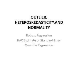
2400 2000 1600 1200 expentidures for durable goods 800 400 0 0 2000 4000 6000 8000 10000 12000 HH-income Example: Household Income and Expenditures 70 households (HH): monthly HH-income and expenditures for durable goods Hackl, Econometrics, Lecture 4
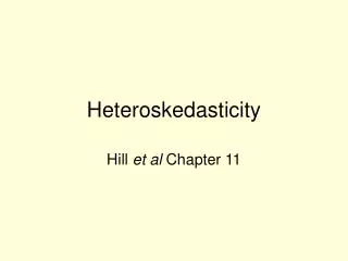
600 400 200 0 residuals e -200 -400 -600 0 2000 4000 6000 8000 10000 12000 HH-income Household Income and Expenditures, cont‘d Residuals e = y- ŷ from Ŷ = 44.18 + 0.17 X X: monthly HH-income Y: expenditures for durable goods the larger the income, the more scattered are the residuals Hackl, Econometrics, Lecture 4
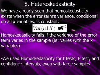
Typical Situations for Heteroskedasticity Heteroskedasticity is typically observed • In data from cross-sectional surveys, e.g., in households or regions • Data with variance which depends of one or several explanatory variables, e.g., firm size • Data from financial markets, e.g., exchange rates, stock returns Hackl, Econometrics, Lecture 4
Example: Household Expenditures With growing income increasing variation of expenditures; from Verbeek, Fig. 4.1 Hackl, Econometrics, Lecture 4
Autocorrelation of Economic Time-series • Consumption in actual period is similar to that of the preceding period; the actual consumption „depends“ on the consumption of the preceding period • Consumption, production, investments, etc.: it is to be expected that successive observations of economic variables correlate positively • Seasonal adjustment: application of smoothing and filtering algorithms induces correlation Hackl, Econometrics, Lecture 4
Example: Imports Scatter-diagram of by one period lagged imports [MTR(-1)] against actual imports [MTR] Correlation coefficient between MTR und MTR(-1): 0.9994 Hackl, Econometrics, Lecture 4
Example: Import Function MTR: Imports FDD: Demand (from AWM-database) Import function: MTR = -227320 + 0.36 FDD R2 = 0.977, tFFD = 74.8 Hackl, Econometrics, Lecture 4
Import Function, cont‘d MTR: Imports FDD: Demand (from AWM-database) RESID: et = MTR - (-227320 + 0.36 FDD) Hackl, Econometrics, Lecture 4
Import Function, cont‘d Scatter-diagram of by one period lagged residuals [Resid(-1)] against actual residuals [Resid] Serial correlation! Hackl, Econometrics, Lecture 4
Typical Situations for Autocorrelation Autocorrelation is typically observed if • a relevant regressor with trend or seasonal pattern is not included in the model: miss-specified model • the functional form of a regressor is incorrectly specified • the dependent variable is correlated in a way that is not appropriately represented in the systematic part of the model Warning! Omission of a relevant regressor with trend implies autocorrelation of the error terms; in econometric analyses autocorrelation of the error terms is always possible! • Autocorrelation of the error terms indicates deficiencies of the model specification • Tests for autocorrelation are the most frequently used tool for diagnostic checking the model specification Hackl, Econometrics, Lecture 4
Import Functions • Regression of imports (MTR) on demand (FDD) MTR = -2.27x10⁹ + 0.357 FDD, tFDD = 74.9, R2 = 0.977 Autocorrelation (order 1) of residuals: Corr(et, et-1) = 0.993 • Import function with trend (T) MTR = -4.45x10⁹ + 0.653 FDD – 0.030x10⁹ T tFDD = 45.8, tT = -21.0, R2 = 0.995 Multicollinearity? Corr(FDD, T) = 0.987! • Import function with lagged imports as regressor MTR = -0.124x10⁹ + 0.020 FDD + 0.956 MTR-1 tFDD = 2.89, tMTR(-1) = 50.1, R2 = 0.999 Hackl, Econometrics, Lecture 4
Consequences of V{e} s2IN OLS estimators b for b • are unbiased • are consistent • have the covariance-matrix V{b} = s2 (X'X)-1 X'YX (X'X)-1 • are not efficient estimators, not BLUE • follow – under general conditions – asymptotically the normal distribution The estimator s2 = e'e/(N-K) for s2 is biased and Hackl, Econometrics, Lecture 4
Consequences of V{e} s2IN for Applications • OLS estimators b for b are still unbiased • Routinely computed standard errors are biased; the bias can be positive or negative • t- and F-tests may be misleading Remedies • Alternative estimators • Corrected standard errors • Modification of the model Tests for identification of • heteroskedasticity • autocorrelation are important tools Hackl, Econometrics, Lecture 4
Contents • Violations of V{ε} = s2 IN • Heteroskedasticity • GLS Estimation • Autocorrelation Hackl, Econometrics, Lecture 4
Inference under Heteroskedasticity Covariance matrix of b: V{b} = s2 (X'X)-1 X'YX (X'X)-1 Use of s2 (X'X)-1 (the standard output of econometric software) instead of V{b} for inference on b may be misleading Remedies • Use of correct variances and standard errors • Transformation of the model so that the error terms are homoskedastic Hackl, Econometrics, Lecture 4
The Correct Variances • V{εi} = σi2= σ2hi2: each observation has its own unknown parameter hi • Nobservation for estimating N unknown parameters? To estimate σ2i – and V{b} • Known form of the heteroskedasticity, specific correction • E.g., hi2 = zi’afor some variables zi • Requires estimation of a • White’s heteroskedasticity-consistent covariance matrix estimator (HCCME) Ṽ{b} = s2(X'X)-1(Siĥi2xixi’) (X'X)-1 with ĥi2=ei2 • Denoted as HC0 • Inference based on HC0: heteroskedasticity-robust inference Hackl, Econometrics, Lecture 4
White’s Standard Errors White’s standard errors for b • Square roots of diagonal elements of HCCME • Underestimate the true standard errors • Various refinements, e.g., HC1 = HC0[N/(N-K)] In GRETL: HC0 is the default HCCME, HC1 and other refinements are optionally available Hackl, Econometrics, Lecture 4
An Alternative Estimator for b Idea of the estimator • Transform the model so that it satisfies the Gauss-Markov assumptions • Apply OLS to the transformed model • Should result in a BLUE Transformation often depends upon unknown parameters that characterizing heteroskedasticity: two-step procedure • Estimate the parameters that characterize heteroskedasticity and transform the model • Estimate the transformed model The procedure results in an approximately BLUE Hackl, Econometrics, Lecture 4
An Example Model: yi = xi’β + εiwith V{εi} = σi2= σ2hi2 Division by hi results in yi /hi = (xi /hi)’β + εi /hi with a homoskedastic error term V{εi /hi} = σi2/hi2= σ2 OLS applied to the transformed model gives It is called a generalized least squares (GLS) or weighted least squares (WLS) estimator Hackl, Econometrics, Lecture 4
Weighted Least Squares Estimator • A GLS or WLS estimator is a least squares estimator where each observation is weighted by a non-negative factor wi > 0: • Weights proportional to the inverse of the error term variance: Observations with a higher error term variance have a lower weight; they provide less accurate information on β • Needs knowledge of the hi • Is seldom available • Is mostly provided by estimates of hi based on assumptions on the form of hi • E.g., hi2 = zi’a for some variables zi • Analogous with general weights wi Hackl, Econometrics, Lecture 4
Example: Labor Demand Verbeek’s data set “labour2”: Sample of 569 Belgian companies (data from 1996) • Variables • labour: total employment (number of employees) • capital: total fixed assets • wage: total wage costs per employee (in 1000 EUR) • output: value added (in million EUR) • Labour demand function labour = b1 + b2*wage + b3*output + b4*capital Hackl, Econometrics, Lecture 4
Labor Demand Function For Belgian companies, 1996; Verbeek Hackl, Econometrics, Lecture 4
Labor Demand Function, cont’d Can the error terms be assumed to be homoskedastic? • They may vary depending of the company size, measured by, e.g., size of output or capital • Regression of squared residuals on appropriate regressors will indicate heteroskedasticity Hackl, Econometrics, Lecture 4
Labor Demand Function, cont’d Auxiliary regression of squared residuals, Verbeek Indicates dependence of error terms on output, capital, not on wage Hackl, Econometrics, Lecture 4
Labor Demand Function, cont’d Estimated function labour = b1 + b2*wage + b3*output + b4*capital OLS estimates without (s.e.) and with White standard errors (White s.e.), and GLS estimates with wi = 1/ei The standard errors are inflated by factors 3.7 (wage), 6.4 (capital), 7.0 (output) wrt the White s.e. Hackl, Econometrics, Lecture 4
Labor Demand Function, cont’d With White standard errors: Output from GRETL Dependent variable : LABOR Heteroskedastic-robust standard errors, variant HC0, coefficient std. error t-ratio p-value ------------------------------------------------------------- const 287,719 64,8770 4,435 1,11e-05 *** WAGE -6,7419 1,8516 -3,641 0,0003 *** CAPITAL -4,59049 1,7133 -2,679 0,0076 *** OUTPUT 15,4005 2,4820 6,205 1,06e-09 *** Mean dependent var 201,024911 S.D. dependent var 611,9959 Sum squared resid 13795027 S.E. of regression 156,2561 R- squared 0,935155 Adjusted R-squared 0,934811 F(2, 129) 225,5597 P-value (F) 3,49e-96 Log-likelihood 455,9302 Akaike criterion 7367,341 Schwarz criterion -3679,670 Hannan-Quinn 7374,121 Hackl, Econometrics, Lecture 4
Tests against Heteroskedasticity Due to unbiasedness of b, residuals are expected to indicate heteroskedasticity Graphical displays of residuals may give useful hints Residual-based tests: • Breusch-Pagan test • Koenker test • Goldfeld-Quandt test • White test Hackl, Econometrics, Lecture 4
Breusch-Pagan Test For testing whether the error term variance is a function of Z2, …, Zp Model for heteroskedasticity si2/s2 = h(zi‘a) with function h with h(0)=1, p-vectors zi und a, an intercept and p-1 variables Z2, …, Zp Null hypothesis H0: a = 0 implies si2 = s2 for all i, i.e., homoskedasticity Auxiliary regression of the standardized squared OLS residuals gi = ei2/s2 - 1, s2 = e’e/N, on zi (and squares of zi) Test statistic: BP = N*ESS with the explained sum of squares ESS = N*V(ĝ), of the auxiliary regression; ĝ are the fitted values for g. BP follows approximately the Chi-squared distribution with pd.f. Hackl, Econometrics, Lecture 4
Breusch-Pagan Test, cont‘d Typical functions h for h(zi‘a) • Linear regression: h(zi‘a) = zi‘a • Exponential function h(zi‘a) = exp{zi‘a} • Auxiliary regression of the log (ei2) upon zi • “Multiplicative heteroskedasticity” • Variances are non-negative • Koenker test: variant of the BP test which is robust against non-normality of the error terms • GRETL: The output window of OLS estimation allows the execution of the Breusch-Pagan test with h(zi‘a) = zi‘a • OLS output => Tests => Heteroskedasticity => Breusch-Pagan • Koenkertest: OLS output => Tests => Heteroskedasticity => Koenker Hackl, Econometrics, Lecture 4
Labor Demand Function, cont’d Auxiliary regression of squared residuals, Verbeek NR2 = 331.04, p-value = 2.17E-70; reject null hypothesis of homoskedasticity Hackl, Econometrics, Lecture 4
Goldfeld-Quandt Test For testing whether the error term variance has values sA2 and sB2 for observations from regime A and B, respectively, sA2 sB2 regimes can be urban vs rural area, economic prosperity vs stagnation, etc. Example (in matrix notation): yA = XAbA + eA, V{eA} = sA2INA (regime A) yB = XBbB + eB, V{eB} = sB2INB (regime B) Null hypothesis: sA2 = sB2 Test statistic: with Si: sum of squared residuals for i-th regime; follows under H0 exactly or approximately the F-distribution with NA-K and NB-Kd.f. Hackl, Econometrics, Lecture 4
Goldfeld-Quandt Test, cont‘d Test procedure in three steps: • Sort the observations with respect to the regimes • Separate fittings of the model to the NA and NB observations; sum of squared residuals SA and SB • Calculation of test statistic F Hackl, Econometrics, Lecture 4
White Test For testing whether the error term variance is a function of the model regressors, their squares and their cross-products Auxiliary regression of the squared OLS residuals upon xi’s, squares of xi’s and cross-products Test statistic: NR2 with R2 of the auxiliary regression; follows the Chi-squared distribution with the number of coefficients in the auxiliary regression as d.f. The number of coefficients in the auxiliary regression may become large, maybe conflicting with size of N, resulting in low power of the White test Hackl, Econometrics, Lecture 4
Labor Demand Function, cont’d White's test for heteroskedasticity OLS, using observations 1-569 Dependent variable: uhat^2 coefficient std. error t-ratio p-value -------------------------------------------------------------- const -260,910 18478,5 -0,01412 0,9887 WAGE 554,352 833,028 0,6655 0,5060 CAPITAL 2810,43 663,073 4,238 2,63e-05 *** OUTPUT -2573,29 512,179 -5,024 6,81e-07 *** sq_WAGE -10,0719 9,29022 -1,084 0,2788 X2_X3 -48,2457 14,0199 -3,441 0,0006 *** X2_X4 58,5385 8,11748 7,211 1,81e-012 *** sq_CAPITAL 14,4176 2,01005 7,173 2,34e-012 *** X3_X4 -40,0294 3,74634 -10,68 2,24e-024 *** sq_OUTPUT 27,5945 1,83633 15,03 4,09e-043 *** Unadjusted R-squared = 0,818136 Test statistic: TR^2 = 465,519295, with p-value = P(Chi-square(9) > 465,519295) = 0,000000 Hackl, Econometrics, Lecture 4
Contents • Violations of V{ε} = s2 IN • Heteroskedasticity • GLS Estimation • Autocorrelation Hackl, Econometrics, Lecture 4
Generalized Least Squares Estimator • A GLS or WLS estimator is a least squares estimator where each observation is weighted by a non-negative factor wi > 0 • Example: yi = xi’β + εiwith V{εi} = σi2= σ2hi2 • Division by hi results in a model with homoskedastic error terms V{εi /hi} = σi2/hi2= σ2 • OLS applied to the transformed model results in the weighted least squares (GLS) estimator with wi = hi-2: • The concept of transforming the model so that Gauss-Markov assumptions are fulfilled is used also in more general situations, e.g., for autocorrelated error terms Hackl, Econometrics, Lecture 4
Properties of GLS Estimators The GLS estimator is a least squares estimator; standard properties of OLS estimator apply • The covariance matrix of the GLS estimator is • Unbiased estimator of the error term variance • Under the assumption of normality of errors, t- and F-tests can be used; for large N, these properties apply approximately without normality assumption Hackl, Econometrics, Lecture 4
Feasible GLS Estimator Is a GLS estimator with estimated weights wi • Substitution of the weights wi = hi-2 by estimatesĥi-2 • Feasible (or estimated) GLS or FGLS or EGLS estimator • For consistent estimates ĥi, the FGLS and GLS estimators are asymptotically equivalent • For small values of N, FGLS estimators are in general not BLUE • For consistently estimated ĥi, the FGLS estimator is consistent and asymptotically efficient with covariance matrix (estimate for s2: based on FGLS residuals) • Warning: the transformed model is uncentered Hackl, Econometrics, Lecture 4
Multiplicative Heteroskedasticity Assume V{εi} = σi2= σ2hi2 = σ2exp{zi‘a} • The auxiliary regression log ei2 = log σ2 + zi‘a + vi with vi = log(ei2/σi2) provides a consistent estimator a for α • Transform the model yi = xi’β + εiwith V{εi} = σi2= σ2hi2 by dividing through ĥi from ĥi2 = exp{zi‘a} • Error term in this model is (approximately) homoskedastic • Applying OLS to the transformed model gives the FGLS estimator for β Hackl, Econometrics, Lecture 4
FGLS Estimation In the following steps: • Calculate the OLS estimates b for b • Compute the OLS residuals ei = yi – xi‘b • Regress log(ei2) on zi and a constant, obtaining estimates a for α log ei2 = log σ2 + zi‘a + vi • Compute ĥi2 = exp{zi‘a}, transform all variables and estimate the transformed model to obtain the FGLS estimators: yi/ĥi = (xi /ĥi)’β + εi/ĥi • The consistent estimate s² for σ2, based on the FGLS-residuals, and the consistently estimated covariance matrix are part of the standard output when regressing the transformed model Hackl, Econometrics, Lecture 4
Labor Demand Function For Belgian companies, 1996; Verbeek Log-tranformation is expected to reduce heteroskedasticity Hackl, Econometrics, Lecture 4
Labor Demand Function, cont’d For Belgian companies, 1996; Verbeek Breusch-Pagan test: NR2 = 66.23, p-value: 1,42E-13 Hackl, Econometrics, Lecture 4
Labor Demand Function, cont’d For Belgian companies, 1996; Verbeek Weights estimated assuming multiplicative heteroskedasticity Hackl, Econometrics, Lecture 4
Labor Demand Function, cont’d Estimated function log(labour)= b1 + b2*log(wage) + b3*log(output)+ b4*log(capital) The table shows: OLS estimates without (s.e.) and with White standard errors (White s.e.) as well as FGLS estimates and standard errors Hackl, Econometrics, Lecture 4
Labor Demand Function, cont’d Some comments: • Reduction of standard errors in FGLS estimation as compared with heteroskedasticity-robust estimation, efficiency gains • Comparison with OLS estimation not appropriate • FGLS estimates differ slightly from OLS estimates; effect of capital is indicated to be relevant (p-value: 0.0086) • R2 of FGLS estimation is misleading • Model is uncentered, no intercept • Comparison with that of OLS estimation not appropriate, explained variable differ Hackl, Econometrics, Lecture 4