Download
1 / 54
550 likes | 966 Views
Signal and Noise. Yongsik Lee. Signal vs. noise. Noise Extraneous and unwanted signals Superimposed on the analyte signal From radio engineering, presence of unwanted signals was noise or static sound. Signal vs. Noise. 5A Signal-to-Noise ratio. S/N

E N D
Signal and Noise Yongsik Lee
Signal vs. noise • Noise • Extraneous and unwanted signals • Superimposed on the analyte signal • From radio engineering, presence of unwanted signals was noise or static sound
5A Signal-to-Noise ratio • S/N • Noise is independent of signal intensity • Absolute noise level is usually constant • Big signal has lower S/N • Better parameter than absolute noise level • Definition • S/N = (mean)/(standard deviation) = <x>/s • <x>/s = 1/RSD
Estimation S/N • S/N (dB) • S/N (dB) = 20 log(S/N) • Confidence level • 주어진 확률로 모집단의 평균이 들어있을 한계 범위를 구한 것 • 신뢰한계 (CL) • 표본표준편차의 크기에 의존 • ±5σ 99% means (max-min) = 5σ • Good S/N • S/N = 2-3 이면 눈으로 관찰 불가능 • Figure 5-2
5B Sources of Noise • Two types of noises in chemical analysis • Chemical noise • 분석하려는 시스템의 화학적 성질에 영향을 주는 변수로부터 • 온도, 압력의 작은 변동 • 상대습도, 진동, 주변 빛의 세기 변화, 실험실내 증기 • 분석물질에 따라 처리 • Instrumental noise • 각 기기 부분에서 나오는 다양한 잡음으로 구성 • Thermal noise • Shot noise • Flicker noise • Environmental noise
Thermal Noise • Johnson Noise • White noise (independent of frequency itself) • Thermal motion of electrons • Will occur even in the absence of a current • T = 0 K, no thermal noise • Rms noise voltage • <ν>rms = (4kTR Δf)1/2 (Volts) • Noise in a frequency bandwidth of Δf (Hz) • K = Boltzmann constant • R = resistance of the resistive element (Ω)
White Noise • Definition • 공기 중에는 수많은 종류의 잡음이 있으며, 이 잡음들은 모든 주파수에서 발생하기 때문에 이러한 잡음을 백색잡음(white noise)이라고 한다. • 주파수가 높은 전자파의 일종인 가시광선이 주파수에 따라 색상이 다르지만 여러 색광이 겹치면 하얀색이 되듯이, 여러 주파수의 잡음이 모인 것이라서 붙여진 의미 • 이와는 반대로 특정 주파수에 집중된 잡음을 유색잡음(Color noise)이라고 부른다.
Rise time and Δf • Δf = 1/(3trise) • Rise time = time for 10% to 90% • Δf decrease means rise time increase • Slow response • Low thermal noise • Temperature and thermal noise • Low temperature
Shot noise • When? Where? • charged particles across junctions • P-n junction • evacuated space between the electrodes • Why? • Quantized random effect • Statistical fluctuation • irms = (2Ie Δf)1/2 • random effect • White noise
Flicker noise • 깜빡이 잡음 • 1/f noise • Frequency dependent noise • Long term drift in dc amplifiers • Significant at f < 100 Hz
Environmental Noise • 환경 잡음 • 기기 주위에서 생기는 다양한 형태의 잡음 • 전자기 복사선을 수신하는 안테나 역할 • Two quiet region • Good quiet region • 1-500 kHz • Fair quiet region • 3-60 Hz
5C Signal-to-Noise Enhancement • Two general methods • Hardware = instrument design • Grounding and shielding • Filter • Chopping • Lock-in, synchronous detection • modulation • Software = algorithm • signal averaging • ADC ed form
Grounding and Shielding • To avoid noise arising electromagnetic radiation • Grounding • Shielding – especially for high resistance transducer • minimizing the lengths of conductors • anntena • Art not science! • Good reference • H.V.Malmstad et. al. • Electronics and instrumentation for scientists • Appendix A
Difference Amplifiers • Common-mode Noise • Generated in the transducer circuit • Appears in an amplified form in the readout • In phase noise • Attenuation using difference amp • Inverting and non-inverting inputs • Noise with same phase disappears • If not enough, use Instrumentation amplifier
Analog Filtering • Remove noise that differs in frequency • Low-pass RC filter • Circuit – Figure 2-11b • Reduce environmental noise • Reduce thermal or shot noise • For a slowly varying dc signal • Figure 5-5 • High-pass filter • Circuit - Figure 2-11a • Reduce drift and other flicker noise • For an ac signal
Narrow band filters • Attenuate noise outside an band of freq • Noise ∝ (Δf)1/2 • Significant noise reduction (NR) • By restricting the input signal to narrow bandwidth
Modulation • 변조/복조 • Mo/dem • Low frequency or dc signals are converted to a higher frequency • 1/f noise is less troublesome at higher freq. • After amplification • Filtering with a high-pass filter to remove 1/f noise • Then amplify dc signal
Chopper Amplifier • Conversion to a square-wave form • Electrical chopper • Mechanical chopper • Example - Atomic Absorption • Use of mechanical chopper • Use high-pass filter • amplification
Lock-in Amplifier • Recovery of signals • Even when S/N = 1 or less • Scheme • Reference signal • Same freq as the signal • Fixed phase difference • Remove high frequency noise • Using low-pass filter
Software Method • Ensemble averaging • 종합적 평균법 • Boxcar averaging • 소집단 평균법 • Digital filtering • 디지털 필터법 • Correlation methods • 상관 관계법
Ensemble averaging • Data in Array format • Successive sets of data stored in memory • Summed point by point (co-addition) • Summed data averaged • Figure 5-9 • S/N increase • Mean Sx = (sum of the individual measurements) / (n, number of measurements) • Mean-square noise = Σ(Sx – Si)2/n • Rms noise = (mean-square noise)1/2 • Variance and standard deviation 이라 불리기도 한다.
S/N for ensemble averaging • S/N • Mean value divided by its standard deviation • = Sx / rms noise • Rms = Root mean square • S/N ∝(n)1/2
Nyquist sampling theorem • Measuring frequency (f) • f ≥ 1/(2Δt) • Where Δt = time interval between the signal samples • At least twice as great as the highest frequency component of the waveform • Example • Signal f = 150 Hz • Sampling rate = at least 300 samples/sec • Customary practice • Sampling at 10 times of Nyquist frequency • Using synchronizing pulse is important to synchronize sampling
Nyquist-Shannon sampling theorem • Background • a fundamental tenet in the field of information theory, in particular telecommunications. • First formulated by Harry Nyquist in 1928 • was only formally proved by Claude E. Shannon in 1949 • The theorem • when converting from an analog signal to digital (or otherwise sampling a signal at discrete intervals), • the sampling frequency must be greater than twice the highest frequency of the input signal • in order to be able to reconstruct the original perfectly from the sampled version. • aliased • If the sampling frequency is less than this limit, then frequencies in the original signal that are above half the sampling rate will be "aliased" and will appear in the resulting signal as lower frequencies. • Therefore, an analog low-pass filter is typically applied before sampling to ensure that no components with frequencies greater than half the sample frequency remain. This is called an "anti-aliasing filter".
Effect of signal averaging • Example of NMR spectra • Figure 5-10 • Random fluctuations in the noise tend to cancel • Signal accumulates • Thus S/N increases
Boxcar averaging • Boxcar averaging • Digital procedures for smoothing irregularities • Enhancing the S/N • The average of small number of adjacent points is a better measure of the signal than any of the individual points • Signal details are lost • Example • Figure 5-11 • Usually 2-50 points are averaged • Done by computer in real time
Boxcar Integrator • Function of boxcar integrator • Boxcar averaging in analog domain • Sample a repetitive waveform • At a programmable time interval • s/n of boxcar integrator • Time constant of the integrator • Scan speed of the sampling window • Aperture time • Time window over which the sampling occurs
Digital Filtering • Types • (Digital) Ensemble averaging • Fourier transformation • Least square polynomial smoothing • correlation
Fourier Synthesis of Waveform • Theory • formulated by the French mathematician Jean Baptiste Joseph Baron Fourier (1768-1830) • any periodic function, no matter how trivial or complex, can be expressed in terms of converging series of combinations of sines and/or cosines, known as Fourier series. • Therefore, any periodic signal is a sum of discrete sinusoidal components.
Square Waveform • Although the calculation of a0, a1, b1, a2, b2, is a mathematically straightforward process, it may become rather tedious depending on the complexity and the discontinuities of f(x) • The Fourier theorem is particularly useful in scientific instrumentation • http://www.chem.uoa.gr/applets/AppletFourier/Appl_Fourier2.html
Fourier transformation • Sinusoidal frequency components • Fourier synthesis of waveform • Non-sinusoidal periodic signals are made up of many discrete sinusoidal frequency components. • Fourier Transform (FT) • The process of obtaining the spectrum of frequencies H(f) comprising a time-dependent signal h(t) • Fourier analysis
Normal and inverse FT • H(f) can be derived from h(t) by employing the Fourier Integral • All FT algorithms manipulate and convert data in both directions, i.e. H(f) can be calculated from h(t) and vice versa
Fast Fourier Transformation • These conversions (for discretely sampled data) are normally done on a digital computer and involve a great number of complex multiplications (N2, for N data points). • Special fast algorithms have been developed for accelerating the overall calculation, • Cooley-Tukey algorithm • known as Fast Fourier Transform (FFT) • With FFT the number of complex multiplications is reduced to Nlog2N. • The difference between Nlog2N and N2 is immense • with N=106 , it is the difference between 0.1 s and 1.4 hours of CPU time for a 300 MHz processor.
Signal Smoothing using FT • Noisy signal in time domain : h(t) • FT generates frequency spectrum H(f) • Selected parts of frequency spectrum can be attenuated or completely removed • These manipulations result into a modified or "filtered" spectrum HΜ(f). • applying FT-1 to HΜ(f) • the modified signal or "filtered" signal hΜ(t) can be obtained.
Fourier Transformation Time domain –(FT)-> frequency domain
Fourier Transformation • Procedures • Time domain to frequency domain • Low pass filter • Remove high frequency (noise) region • Inverse FT (FT-1) • Usage • FT-IR, FT-NMR • Fast computer
Least-squares polynomial • m-point unweighted smooth • Moving average algorithm • Simpler software technique for smoothing signals consisting of equidistant points • Smoothing width = m 개의 점을 평균하여 (m+1)/2 위치에 표시 • An array of raw (noisy) data [y1, y2, …, ym] can be converted to a new array of smoothed data. • The S/N may be further enhanced by increasing the filter width or by smoothing the data multiple times.
Advantages of moving Average • Reduction of noise • act as a low pass filter • Modest S/N enhancement • Smoothing variables may be determined after data collection • Type of smooth, smooth width, number of times that the data are smoothed • Requires minimal computer time
Disadvantages of moving average • Obviously after each filter pass the first n and the last n points are lost. • Moving average algorithm is particularly damaging when the filter passes through peaks that are narrow compared to the filter width. • information is lost and/or distorted • because too much statistical weight is given to points that are well removed from the central point.
Savitzky-Golayalgorithm • A least squares fit of a small set of consecutive data points to a polynomial and • calculated central point of the fitted polynomial curve as the new smoothed data point. • A. Savitzky and M. J. E. Golay, Anal. Chem., 1964, 36, 1627 • Convolution integers • a set of integers (A-n, A-(n-1) …, An-1, An) could be derived and used as weighting coefficients to carry out the smoothing operation. • exactly equivalent to fitting the data to a polynomial, as just described and it is computationally more effective and much faster
Calculation of Derivatives • calculating the derivatives of noisy signals • Sets of convolution integers can be used to obtain directly its 1st, 2nd, …, m-th order derivative • Figure 5-14 • Savitzky-Golay algorithm is very useful for calculating the derivatives of noisy signals consisting of discrete and equidistant points. • The smoothing effect of the Savitzky-Golay algorithm • not so aggressive as in the case of the moving average • the loss and/or distortion of vital information is comparatively limited. • However, it should be stressed that both algorithms are "lossy", i.e. part of the original information is lost or distorded.