Download
1 / 33
330 likes | 433 Views
Wind power is a growing source of renewable energy, converting wind energy into electricity through turbines. As of 2008, global capacity reached 121.2 gigawatts, accounting for 1.5% of worldwide electricity, with notable penetration in Denmark (19%), Spain and Portugal (11%), and Germany and Ireland (7%). Studies indicate that the potential for wind energy output could exceed five times current global energy consumption with 72 TW of theoretical capacity. Overcoming economic and environmental barriers is essential for realizing this vast potential.

E N D
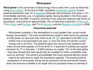
Wind power Wind power is the conversion of wind energy into a useful form, such as electricity, using wind turbines. At the end of 2008, worldwide nameplate capacity of wind-powered generators was 121.2 gigawatts.Although wind produces only about 1.5% of worldwide electricity use, it is growing rapidly, having doubled in the three years between 2005 and 2008. In several countries it has achieved relatively high levels of penetration, accounting for approximately 19% of electricity production in Denmark, 11% in Spain and Portugal, and 7% in Germany and the Republic of Ireland in 2008. Theoretical potential Wind power available in the atmosphere is much greater than current world energy consumption. The most comprehensive study to date found the potential of wind power on land and near-shore to be 72 TW, equivalent to 54,000 MToE (million tons of oil equivalent) per year, or over five times the world's current energy use in all forms. The potential takes into account only locations with mean annual wind speeds ≥ 6.9 m/s at 80 m. It assumes 6 turbines per square kilometer for 77 m diameter, 1.5 MW turbines on roughly 13% of the total global land area (though that land would also be available for other compatible uses such as farming). The authors acknowledge that many practical barriers would need to be overcome to reach this theoretical capacity. The practical limit to exploitation of wind power will be set by economic and environmental factors, since the resource available is far larger than any practical means to develop it.
Evaluation of global wind power by Cristina L. Archer and Mark Z. Jacobson
Evaluation of global wind power by Cristina L. Archer and Mark Z. Jacobson
Evaluation of global wind power by Cristina L. Archer and Mark Z. Jacobson
Theoretical potential -conclusions • Approximately 13% of all stations worldwide belong to class 3 or greater (i.e., annual mean wind speed ≥ 6.9 m/s at 80 m) and are therefore suitable for wind power generation. This estimate is conservative, since the application of the LS methodology to tower data from the Kennedy Space Center exhibited an average underestimate of -3.0 and -19.8% for sounding and surface stations respectively. In addition, wind power potential in all areas for which previous studies had been published was underestimated in this study. • The average calculated 80-m wind speed was 4.59 m/s (class 1) when all stations are included; if only stations in class 3 or higher are counted, the average was 8.44 m/s (class 5). For comparison, the average observed 10-m wind speed from all stations was 3.31 m/s (class 1) and from class ge 3 stations was 6.53 m/s (class 6). • Europe and North America have the greatest number of stations in class = 3 (307 and 453, respectively), whereas Oceania and Antarctica have the greatest percentage (21 and 60%, respectively). Areas with strong wind power potential were found in Northern Europe along the North Sea, the southern tip of the South American continent, the island of Tasmania in Australia, the Great Lakes region, and the northeastern and western coasts of Canada and the United States.
Theoretical potential -conclusions • Offshore stations experience mean wind speeds at 80 m that are ~90% greater than over land on average. • The globally-averaged values of the friction coefficient a and the roughness length z0 are 0.23-0.26 and 0.63-0.81 m, respectively. Both ranges are larger than what is generally used (i.e., a=0.14 and z0=0.01 m) and are more representative of urbanized/rough surfaces than they are of grassy/smooth ones. • The globally-averaged 80-m wind speed from the sounding stations was higher during the day (4.96 m/s) than night (4.85 m/s). Only above ~120 m the average nocturnal wind speed was higher than the diurnal average. • Global wind power potential for the year 2000 was estimated to be ~72 TW (or ~54,000 Mtoe). As such, sufficient wind exists to supply all the world?s energy needs (i.e., 6995-10177 Mtoe), although many practical barriers need to be overcome to realize this potential.
WIND ENERGY CONVERSION SYSTEMS • Power is transferred from the wind to the rotor then passed through the gearbox, generator, and power electronics until it finally reaches the gird. • Each stage of the power transfer has a certain efficiency. Therefore, each power transfer stage presents an opportunity to reduce the cost of energy from a wind turbine.
The Wind turbine • The figure to the right shows the general parts of a wind turbine. • The rotor of modern wind turbines typically have three blades. • The nacelle yaws or rotates on the tower to keep the turbine faced into the wind. • The nacelle houses the gear box and generator.
Betz’ law It shows the maximum possible energy — known as the Betz limit — that may be derived by means of an infinitely thin rotor from a fluid flowing at a certain speed peed. In order to calculate the maximum theoretical efficiency of a thin rotor (of, for example, a wind mill) one imagines it to be replaced by a disc that withdraws energy from the fluid passing through it. At a certain distance behind this disc the fluid that has passed through flows with a reduced velocity. Schematic of fluid flow through a disk-shaped actuator.
Betz’ law Assumptions 1. The rotor does not possess a hub, this is an ideal rotor, with an infinite number of blades which have 0 drag. Any resulting drag would only lower this idealized value. 2. The flow into and out of the rotor is axial. This is a control volume analysis, and to construct a solution the control volume must contain all flow going in and out, failure to account for that flow would violate the conservation equations. 3. This is incompressible flow. The density remains constant, and there is no heat transfer from the rotor to the flow or vice versa. Applying conservation of mass to this control volume, the mass flow rate (the mass of fluid flowing per unit time) is given by: (1) where v1 is the speed in the front of the rotor and v2 is the speed downstream of the rotor, and v is the speed at the fluid power device. ρ is the fluid density, and the area of the turbine is given by S.
Betz’ law The force exerted on the wind by the rotor may be written as (2) and the power content in the wind is (3) However, power can be computed another way, by using the kinetic energy. Applying the conservation of energy equation to the control volume yields (4) Both of these expressions for power are completely valid, one was derived by examining the incremental work done and the other by the conservation of energy. Equating these two expressions yields (5)
Betz’ law (6) The work rate obtainable from a cylinder of fluid with area S and velocity v1is: (7) hence (8)
Betz’ law (9) (10)
Fixed Speed Vs Variable Speed Rotor • The figure above compares the percentage of available wind power(Betz’s Limit already accounted for) that a fixed speed rotor and variable speed rotor can capture at each wind speed. • The variable speed captures more energy at almost all wind speeds. However, the power electronics needed for a variable speed system are costly and take away some of the efficiency gains. Whether the variable speed systemis worth the extra cost depends on the sites wind speed distribution.
Wind Turbine Blade Analysis using the BladeElement Momentum Method Axial Stream tube around a Wind Turbine Four stations are shown in the diagram: 1, some way upstream of the turbine, 2 just before the blades, 3 just after the blades and 4 some way downstream of the blades. Between 2 and 3 energy is extracted from the wind and there is a change in pressure as a result.
Wind Turbine Blade Analysis using the BladeElement Momentum Method • Assume p1 = p4 and that V2 = V3. We can also assume that between 1 and 2 • and between 3 and 4 the flow is frictionless so we can apply Bernoulli’s equation. (11) Assuming also (12) yields (13)
Wind Turbine Blade Analysis using the BladeElement Momentum Method Noting that force is pressure times area we find that: (12) Define the axial induction factor as: (13) It can also be shown that: (14) Substituting yields: (15)
Wind Turbine Blade Analysis using the BladeElement Momentum Method Consider the rotating annular stream tube shown in Figure 2. Four stations are shown in the diagram 1, some way upstream of the turbine, 2 just before the blades, 3 just after the blades and 4 some way downstream of the blades. Between 2 and 3 the rotation of the turbine imparts a rotation onto the blade wake.
Wind Turbine Blade Analysis using the BladeElement Momentum Method Consider the conservation of angular momentum in this annular stream tube. The blade wake rotates with an angular velocity w and the blades rotate with an angular velocity of W. Recall from basic physics that: Moment of Inertia of an annulus, (16) (17) Angular moment, Torque, (18) (19)
Wind Turbine Blade Analysis using the BladeElement Momentum Method Rotating Annular Stream tube: notation. The Blade Element Model
Wind Turbine Blade Analysis using the BladeElement Momentum Method So for a small element the corresponding torque will be: (20) For the rotating annular element (21) (22) Define angular induction factor : (23) Recall that (24)
Wind Turbine Blade Analysis using the BladeElement Momentum Method • Blade element theory relies on two key assumptions: • There are no aerodynamic interactions between different blade elements • The forces on the blade elements are solely determined by the lift and drag • coefficients Consider a blade divided up into N elements. Each of the blade elements will experience a slightly different flow as they have a different rotational speed (Ωr), a different chord length (c) and a different twist angle (γ). Blade element theory involves dividing up the blade into a sufficient number (usually between ten and twenty) of elements and calculating the flow at each one. Overall performance characteristics are determined by numerical integration along the blade span.
Wind Turbine Blade Analysis using the BladeElement Momentum Method Relative flow Flow onto the turbine blade
Wind Turbine Blade Analysis using the BladeElement Momentum Method Lift and drag coefficient data area available for a variety of aerofoils from wind tunnel data. Since most wind tunnel testing is done with the aerofoil stationary we need to relate the flow over the moving aerofoil to that of the stationary test. To do this we use the relative velocity over the aerofoil. More details on the aerodynamics of wind turbines and aerofoil selection can be found in Hansen and Butterfield (1993). In practice the flow is turned slightly as it passes over the aerofoil so in order to obtain a more accurate estimate of aerofoil performance an average of inlet and exit flow conditions is used to estimate performance. The flow around the blades starts at station 2 and ends at station 3. At inlet to the blade the flow is not rotating, at exit from the blade row the flow rotates at rotational speedω. That is over the blade row wake rotation has been introduced. The average rotational flow over the blade due to wake rotation is therefore ω/2. The blade is rotating with speed Ω. The average tangential velocity that the blade experiences is therefore Ωr+ 1/2ωr. (25) The value of βwill vary from blade element to blade element
Wind Turbine Blade Analysis using the BladeElement Momentum Method The local tip speed ratio is defined as (26) Forces on the turbine blade
Wind Turbine Blade Analysis using the BladeElement Momentum Method So the expression for tanβ can be further simplified: (27) And hence the relative velocity is (28) note that by definition the lift and drag forces are perpendicular and parallel to the incoming flow. For each blade element one can see: (29) where dL and dD are the lift and drag forces on the blade element respectively. dL and dD can be found from the definition of the lift and drag coefficients as follows: (30)
Wind Turbine Blade Analysis using the BladeElement Momentum Method This graph shows that for low values of incidence the aerofoil successfully produces a large amount of lift with little drag. At around i = 14º a phenomenon known as stall occurs where there is a massive increase in drag and a sharp reduction in lift. Lift and Drag Coefficients for a NACA 0012 Aerofoil
Wind Turbine Blade Analysis using the BladeElement Momentum Method If there are B blades the forces are calculated as (31) The Torque on an element, dT is simply the tangential force multiplied by the radius. (32) The effect of the drag force is clearly seen in the equations, an increase in thrust force on the machine and a decrease in torque (and power output) These equations can be made more useful by noting that b and W can be expressed in terms of induction factors (33) where σ’ is called the local solidity and is defined as: (34)
Wind Turbine Blade Analysis using the BladeElement Momentum Method Tip Loss Correction Blade tip vortices remain close to the rotor and to the following blades for several rotor revolutions=>a strongly three-dimensional induced velocity field=>fluctuating air loads on the blade=>affecting the rotor performance & source of vibration and noise
Wind Turbine Blade Analysis using the BladeElement Momentum Method Tip Loss Correction At the tip of the turbine blade losses are introduced in a similar manner to those found in wind tip vorticies on turbine blades. These can be accounted for in BEM theory by means of a correction factor. This correction factor Q varies from 0 to 1 and characterises the reduction in forces along the blade. (35) The results from cos-1must be in radians.
Wind Turbine Blade Analysis using the BladeElement Momentum Method Tip Loss Correction The tip loss correction is applied to the axial force and torque as (36) Blade Element Momentum Equations We now have four equations, two dervied from momentum theory which express the axial thrust and the torque in terms of flow parameters Eq.36 (33) To calculate rotor performance Equations 36 from a momentum balance are equated with Equations 33. Once this is done the following useful relationships arise: (34)
Wind Turbine Blade Analysis using the BladeElement Momentum Method Power Output The contribution to the total power from each annulus is: (35) The total power from the rotor is: (36) Where rhis the hub radius. The power coefficient CPis given by: (37) Using Equation 33 it is possible to develop an integral for the power coefficient directly. After some algebra: (38)