Designing Effective Monitoring Programs for Fish Population Response to Habitat Restoration

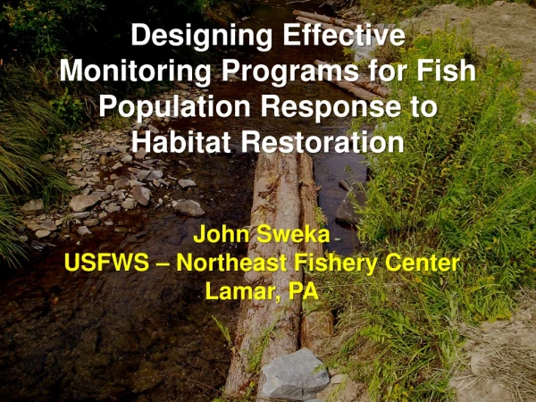
1. Designing Effective Monitoring Programs for Fish Population Response to Habitat Restoration John Sweka USFWS – Northeast Fishery Center Lamar, PA

3. What is the goal of fish habitat restoration efforts and partnerships? To create more/better fish habitat To enhance/recover/restore fish populations

4. How do we know if we met our goal? We need to monitor

5. Adaptive Management DOI Technical Guide Example Models: More Large Woody Debris = More Brook Trout Lower Sediment Load = More Brook Trout

6. Issues of spatial scale • Defining the population of interest • Depends on the goal of the habitat restoration work • Reach population vs. stream population vs. range wide population • Often a mismatch between the population of interest and spatial scale of habitat restoration and monitoring • Can lead to erroneous conclusions about the effectiveness of habitat restoration

7. 300 m Brook trout abundance A0 = 15 A1 = 30 100% increase !!!!!!

8. 300 m 6000 m If abundance throughout the rest of the steam stays the same, this is only a 5% increase.

9. Issues of spatial scale • Life history information can inform decisions on spatial scale of monitoring • Home range – Does monitoring encompass the home range of individuals in the population? • Schooling behavior – Is the species of interest patchily distributed? • Migration – Does the species of interest migrate from one habitat to another while completing its life cycle?

10. A good example of monitoring at the population scale Liermann, M. and P. Roni. 2008. More sites or more years? Optimal study design for monitoring fish response to watershed restoration. North American Journal of Fisheries Management 28: 935-943. “…the only way to assess the population level effects of watershed scale restoration is to monitor at the population level.” Monitored salmon smolt migration from small streams with and without habitat restoration. Employed knowledge of life history information (migration) Replicated experiment with controls

11. Issues of temporal scale How does the duration of monitoring compare to the life history of the species of interest? Generation Time – amount of time it takes one cohort to grow up and replace another; can be calculated from a life table or a Leslie matrix Population growth rate(λ) = 1.6, generation time = 2.14

12. Issues of temporal scale If habitat restoration has a population level effect, we would not expect to begin seeing any real change until the expected generation time is reached Likely longer due to variation in other uncontrollable factors (e.g. rainfall, flow, temperature, predation etc.) Length of monitoring can greatly influence conclusions that are drawn

13. Sweka , J.A. and K.J. Hartman. 2006. Effects of large woody debris addition on stream habitat and brook trout populations in Appalachian streams. Hydrobiologia 559: 363-378.

14. Sweka , J.A. and K.J. Hartman. 2006. Effects of large woody debris addition on stream habitat and brook trout populations in Appalachian streams. Hydrobiologia 559: 363-378.

15. Types of Monitoring Designs Before-After Design Abundance Best if there is many years of pre- and post- data Simply compare pre- and post- mean abundance Time Assumes everything but the treatment remained constant through time

16. Types of Monitoring Designs Pre/Post Pairs Abundance Allows assessment of site-to-site variation Temporal scale may not be long enough Ignores any regional trends in abundance that may exist Time

17. Types of Monitoring Designs Before-After-Control-Impact Design (BACI) Control site Abundance Treatment site Has an independent control site Best if there are several years of pre- and post- data Interested in the difference between treatment and control Embraces natural variation Time

18. Types of Monitoring Designs Before-After-Control-Impact Design (BACI) Treatment site Abundance Control site Control can have higher or lower abundance than the treatment site Time

19. Types of Monitoring Designs Before-After-Control-Impact Design (BACI) Control sites Treatment sites Abundance Can have several treatment and control sites Time

20. Types of Monitoring Designs Real World Case Abundance Control site Treatment site Limited funding, 1 year pre-, couple years post- Time Add a control – separate natural variation from treatment variation Continue monitoring treatment and control – look for treatment x time interaction

21. Power and Sample Size • Power – the probability of correctly rejecting the null hypothesis of no change (no difference) when some specified alternative is correct • How much Power do you need? • Depends on the consequences • Law of diminishing returns – rate of increase in power decreases with increasing sample size • Increasing power can be costly

22. Power and Sample Size • How many samples should I take to detect a difference? • Choice of alpha (chance of falsely rejecting Ho) • Whether the test will be one- or two-tailed • Value of the alternative Ha(desired difference to detect) • Choice of design • Some assumption about the behavior of the variation in the data (e.g variance proportional to mean) • Estimate of the variation (standard deveiation or variance)

23. Power and Sample Size Guidelines for choosing an effect size (Gerow 2007) Small Effect – the smallest difference that elicits your interest Large Effect – the smallest difference that you would definitely not want to fail to detect Medium Effect - the average of small and large effects

24. Power and Sample Size Gerow, K. G. 2007. Power and sample size estimation techniques for fisheries management: Assessment and a new computational tool. North American Journal of Fisheries Management 27: 397 – 404. Gerrodette, T. 1987. A power analysis for detecting trends. Ecology 68: 1364-1372.

25. Conclusions • Effective monitoring starts with a clearly defined population of interest and goals • Incorporate the life history, home range, and behavior of the target species • Have a control and avoid psuedoreplication • View monitoring as an experiment (hypothesis testing) • Use power analysis to inform study design • Funding timelines don’t match biological timelines • Additional partnerships • Creative ways to extend funding • Work with funding sources for change

26. Questions??