Download
1 / 48
480 likes | 689 Views
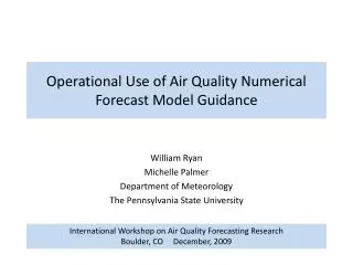
Operational Use of Air Quality Numerical Forecast Model Guidance. William Ryan Michelle Palmer Department of Meteorology The Pennsylvania State University. International Workshop on Air Quality Forecasting Research Boulder, CO December, 2009. What Do We Forecast?.

E N D
Operational Use of Air Quality Numerical Forecast Model Guidance William Ryan Michelle Palmer Department of Meteorology The Pennsylvania State University International Workshop on Air Quality Forecasting Research Boulder, CO December, 2009
What Do We Forecast? Forecasts are verified by peak 8-hour averaged O3 at location of state and local monitors While model forecast location of peak O3 is of interest, air quality alert applies to entire metropolitan area in order to reduce emissions as well as protect health
Complex Land-Sea Boundary Effects Numerical O3 models (NAQC shown at right) often forecast high O3 along land-sea boundaries. These areas of high concentrations can “bleed” inland. First Order Post-Processing: Restrict domain peak O3 guidance to location of monitors. Can retrieve “point” data quickly from www/weather.gov/aq using Firefox
Philadelphia O3 Monitor Network (2007-2009) NAQC “Forecast” is peak 8-h O3 at location of monitors. Addition of “proxy” monitors in locations with less dense coverage does not affect results.
Numerical Forecast Model Guidance: NAQC Model Changes During Period of Interest Emissions Updated Yearly (May) NAQC Upgrade : Sept, 2007 (Experimental Operational) BC, ACM PBL, NAM photolysis NAM Upgrade: Mar, 2008 (horizontal advection, AIRS radiance, soil moisture) NAM Upgrade: Dec, 2008 (GDAS, absorption coefficient water, ice)
NAQC Forecast Skill in PHL 2007-2008 NAQC Forecast Error for PHL Area (2007-2008)
Ladder of Simple Post Processing in the Operational Environment Details? In-Depth Slides: Topic 1
Results of Bias, Trend and Ensemble Methods • All methods showed slight improvement in overall skill. Bias removed, mean absolute error improvement from 0-9%. • 2-Day Running Bias Correction reduced False Alarms with only slight reduction of the Hit Rate. • NB: 2009 may be ananomolous O3 season (In Depth Slides: Topic 2)
Temperature and NAQC Forecast Guidance Peak O3 concentrations, either forecast or observed, are correlated to Tmax. NAQC forecasts (2009 shown left) appear to be sensitive atTmax > 82⁰F Evidence of decoupling of Tmax-O3 association in recent years? In-Depth Slides: Topic 3
Transported O3and NAQC Forecast Guidance IR Channel 4 1515 UTC August 4 Hourly O3 in PHL on August 5 Peak 8-h Ave: 69 ppbv Back Trajectories Initialized 1200 UTC August 4, 24-h Duration, Terminate at 1500 (red), 1000 (blue) and 500 (green) m AGL.
Temperature and Persistence Adjustment • Fit regression model with observed O3 (2007-2008) as predicand, Tmax, persistence O3 and NAQC forecast O3 as predictors. • Modest improvement overall but large reduction in false alarms with only minor reduction in hit rate. Details? In-Depth Slides: Topic 4
2009 Results “NAQC” is uncorrected model forecast, “TempC” is temperature and persistent adjusted forecast, “2dBC” is running two-day bias correction, “Forecast” is expert forecast issued to public.
Summary • Metric of interest to forecasters is peak domain wide O3 and particularly at the threshold of 76 ppbv (Code Orange). • Numerical model forecasts in PHL are skillful but suffer from over-prediction at the Code Orange threshold. • Overall forecast skill is improved by running bias corrections. • Skill at Code Orange threshold improved by excluding coastal regions and correcting for temperature and persistence O3. • Another year of data is necessary to fully test these conclusions due to unusual circumstances in 2009.
Acknowledgements • Air quality forecasting and research in the Philadelphia Metropolitan area is supported by the Delaware Valley Regional Planning Commission (www.dvrpc.org) and the States of PA, NJ and DE. • Additional research support was provided by the Air and Radiation Management Administration of the Maryland Department of the Environment (http://www.mde.state.md.us).
In Depth Slides • Topic 1: Post Processing of Numerical Guidance • Topic 2: Comments on the 2009 Ozone Season in the mid-Atlantic • Topic 3: Temperature-Ozone Relationship Following the NOx SIP Rule Implementation • Topic 4: Using Temperature and Persistence O3 to Adjust NAQC Forecasts
In Depth Slides: Topic 1Post-Processing of Numerical Guidance • Simple bias correction (BC) • Bin forecasts by concentration and correct for historical bias in those ranges. • Running bias correction (RBC) • 2 day running bias correction. • Trend correction • Add recent trend in forecast O3 to current day observed O3 • Blend with statistical models • “Poor Man’s Ensemble” • Statistical post-processing • Predictors: Forecast, temperature and persistence O3
2009 Bias Corrected Forecasts N = 143 r = 0.82 r2 = 0.67 [O3] = 3.52 + 0.89*[O3]BC Overall absolute error similar to uncorrected forecast. No improvement in higher end of observed O3 distribution.
Running Bias Correction (Two Day) • RB O3 = fd+1 - [((fd0 – obsd0) + (fd-1 - obsd-1))/2] • Current day (do) O3 must be estimated from early afternoon observations. • Running bias correction is the average forecast bias over two days preceding the forecast day. • “f” is peak 8-hour O3 forecast at monitor locations by the NAQC model. “obs” is observed peak 8-hour O3 from same locations.
Two-Day Running Bias Correction 2007-2009 N = 406 r = 0.80 r2 = 0.64 [O3] = 14.4 + 0.76*[O3]2dBias Overall, little change in absolute error from NAQC. Some improvement in bias. In 75th%ile (> 65 ppbv), slight degradation in absolute error.
Trend Correction • Trend Corrected O3 = (obsd0 + [fcd+1 – fcd0]) • Today’s Peak O3 + [Tomorrow’s Forecast O3 – Yesterday’s Forecast O3 for Today] • Shortcoming: Forecast is issued before today’s peak observed O3 is known. • Current day forecast from either 0600 or 1200 UTC NAQC runs have not proven reliable so current day peak is typically extrapolated from early afternoon O3 observations.
Trend Correction Results (2007-2009) 2007-2009 N = 409 r = 0.79 r2 = 0.62 [O3] = 17.2 + 0.72*[O3]Trend Overall, little improvement to NAQC forecast.
Blend of Statistical and Numerical Models • Statistical models typically use meteorological, seasonal and persistence predictors to forecast peak domain-wide O3. • These models are simple and cost-effective and have historically provided reasonably accurate forecast guidance. • Statistical models require relatively long training data sets. Usually 5 or more summer seasons of data. • Significant changes in regional scale NOx emissions beginning in 2002 due to the “NOx SIP Rule” have had an impact on the skill of statistical models that are “tuned” to earlier years.
Statistical Model Bias (2003-2009) Bias in forecasts of peak domain-wide 8-hour O3 by two models used in PHL and trained on pre-NOx SIP Rule historical data.
Newest Statistical Model (Trained on Post-NOx SIP Rule data) Improves Performance
Weighted Blend of Statistical and Numerical Models 2009 N = 143 NAQC Blend r 0.83 0.85 r2 0.68 0.73 NAQFS: [O3] = 8.5 + 0.78 * [O3]FC Blend: [O3] = 2.0 + 0.87 * [O3]FC Blend 3: 30% R2009 (post-NOx SIP), 20% R0302 (pre-NOx SIP), 50% NAQFS
In Depth Slides: Topic 2Comments on the 2009 O3 Season • 2009 was a very unusual summer. Low frequency of O3 conducive weather locally and regionally. • “Standard” high O3 weather – westward extension of the Bermuda High, sustained westerly transport from the Ohio River Valley – was infrequent. • This weather pattern contributed to historically low frequency of high O3 cases but there may have been lower emissions due to economic recession.
Mean Summer Upper Air Pattern Featured a Strong and Persistent Area of Low Pressure in Eastern Canada Mean 500 mb Geopotential Height June-August Climate figures courtesy of NOAA-CDC, http://www.cdc.noaa.gov/data/composites/day/
Boundary Layer (925 mb) Mean Winds For June-August, mean winds (left panel) are NW for PHL and northeastern US. Change from normal (right panel) show stronger winds with northerly component
This Resulted in Very Cool Boundary Layer Temperatures Across the Northeast Mean 925 mb Temperature For JJA (left panel). Departure from normal (bottom panel).
The northern US was quite cool in June and July with slightly higher than normal precipitation
Philadelphia Summer Weather • Average temperature for MJJA was near normal. However, June and July were 1.5°F below normal. • August had an average number of hot days (≥ 90°F) but MJJ had only 5 hot days compared to ≈ 11 on average. • All months had more than average number of days with measureable precipitation (17 days in June alone). For the season, 14 additional days of measureable rain (≥ 0.01”). • August was excessively wet with 10.3” of rain, primarily due to 5 days with > 1” of rain (average is 1.2 days).
Weather and Air Quality • The combination of cooler and wetter than normal weather, and the absence of persistent Bermuda High circulation, led to lower than normal O3 regionally and locally • Shenandoah National Park has historically low frequency of high O3 days. • PM2.5 concentrations in PHL very low - pointing to few “dirty” air mass episodes. • Almost no high O3 episodes in Philadelphia.
Philadelphia: Frequency of High O3 Days(Peak 8-Hour O3 in the Metropolitan Area)
Shenandoah National ParkNumber of Days with 8-Hour O3 Above Thresholds
Shenandoah National Park – Big MeadowsRegional Effect of NOx Reductions No days in excess of 70 ppbv in 2009
PHL PM2.5 Concentrations Remarkably Low in 2009 Note: Data for 2004-2008 uses gravimetric filter monitors (FRM) while 2009 uses 24-average from continuous monitors.
Philadelphia: Number of Days with PM2.5 (Daily Average in μgm-3) Above Given Threshold
Shenandoah NP PM2.5 Daily Average Concentrations (May-August, 2004-2009)
In Depth Slides: Topic 3Changes in the Temperature-Ozone Relationship • O3 concentrations are strongly associated with surface temperature (Tmax) • Hot weather is necessary, but not sufficient for high O3 • Since the implementation of the NOxSIP Rule emissions controls, the likelihood of “bad” air given hot temperature has decreased. • This has impacted the skill of both numerical and statistical forecast models.
Philadelphia Ozone- Temperature Relationship Peak 8-Hour O3 in metropolitan PHL and Tmax (PHL Int’l Airport) for May-Sept, 1993-2009
Hot Weather is Necessary but not Sufficient for High O3 If Tmax is ≥ 90⁰F, what is the chance of Code Orange (≥ 76 ppbv) or Code Red (≥ 96 ppbv) O3 occurring?
O3 – Temperature Relationship in PHL: NOxSIP Rule Pre-NOx Rule
In Depth Slides: Topic 4Using Temperature and Persistence O3 to Post-Process NAQC Guidance • Using 2007-2008 data, fit observed O3 and NAQC forecast with two models: • NREG01: NAQC and Tmaxas predictors • NREG02: NAQC, Tmax and LagO3as predictors • As applied to 2009 data, both models gave an increase in skill • Reduced “false alarms” of high O3 by two thirds. • With no reduction in probability of detection.
Simple Post-Processing Method[O3]obs = f([O3]forecast, [O3]persistence, Tmax) 2007-2008 N = 268 r = 0.79 r2 = 0.62 [O3]obs = 0.56 * [O3]NAQC + 0.44 * Tmax + 0.17 * [O3]lag -20.1 Modest improvement in explained variance and correlation
Fit to Observations in 2009 Hit Rate unchanged but number of False Alarms reduced from 14 to 5. 3 of 5 False Alarms are “near misses” with observed O3 ≥ 71 ppbv.