Download
1 / 40
550 likes | 933 Views
CSE 337: Introduction to Medical Imaging Lecture 6: X-Ray Computed Tomography. Klaus Mueller Computer Science Department Stony Brook University. Overview. Scanning: rotate source-detector pair around the patient. data. reconstruction routine. reconstructed cross-sectional slice.

E N D
CSE 337: Introduction to Medical ImagingLecture 6: X-Ray Computed Tomography Klaus Mueller Computer Science Department Stony Brook University
Overview Scanning: rotate source-detector pair around the patient data reconstruction routine reconstructed cross-sectional slice sinogram: a line for every angle
Early Beginnings film Linear tomography only line P1-P2 stays in focus all others appear blurred Axial tomography in principle, simulates the backprojection procedure used in current times
Current Technology • Principles derived by Godfrey Hounsfield for EMI • based on mathematics by A. Cormack • both received the Nobel Price in medizine/physiology in 1979 • technology is advanced to this day • Images: • size generally 512 x 512 pixels • values in Hounsfield units (HU) in the range of –1000 to 1000 m: linear attenuation coefficient: mair= -1000 mwater= 0 mbone = 1000 • due to large dynamic range, windowing must be used to view an image
CT Detectors • Scintillation crystal with photomultiplier tube (PMT) (scintillator: material that converts ionizing radiation into pulses of light) • high QE and response time • low packing density • PMT used only in the early CT scanners • Gas ionization chambers • replace PMT • X-rays cause ionization of gas molecules in chamber • ionization results in free electrons/ions • these drift to anode/cathode and yield a measurable electric signal • lower QE and response time than PMT systems, but higher packing density • Scintillation crystals with photodiode • current technology (based on solid state or semiconductors) • photodiodes convert scintillations into measurable electric current • QE > 98% and very fast response time
Projection Coordinate System • The parallel-beam geometry at angle represents a new coordinate system (r,s) in which projection I(r) is acquired • rotation matrix R transforms coordinate system (x, y)to (r, s): that is, all (x,y) points that fulfill r = x cos( ) + y sin() are on the (ray) line L(r,) • RT is the inverse, mapping (r, s) to (x, y) s is the parametric variable along the (ray) line L(r,)
Projection • Assuming a fixed angle , the measured intensity at detector position r is the integrated density along L(r,): • For a continuous energy spectrum: • But in practice, is is assumed that the X-rays are monochromatic
Projection Profile • Each intensity profile I(r) is transformed to into an attenuation profile p(r): • p(r) is zero for |r|>FOV/2 (FOV = Field of View, detector width) • p(r) can be measured from (0, 2) • however, for parallel beam views (, 2) are redundant, so just need to measure from (0, ) I(r) p(r)
Sinogram • Stacking all projections (line integrals) yields the sinogram, a 2D dataset p(r,) • To illustrate, imagine an object that is a single point: • it then describes a sinusoid in p(r,): projections point object sinogram
Radon Transform • The transformation of any function f(x,y) into p(r,) is called the Radon Transform • The Radon transform has the following properties: • p(r,) is periodic in with period 2p • p(r,) is symmetric in with period p
Dr Ds D Sampling (1) • In practice, we only have a limited • number of views, M • number of detector samples, N • for example, M=1056, N=768 • This gives rise to a discrete sinogram p(nDr,mD) • a matrix with M rows and N columns Dr is the detector sampling distance D is the rotation interval between subsquent views • assume also a beam of width Ds • Sampling theory will tell us how to choose these parameters for a given desired object resolution
Sampling (2) spatial domain frequency domain projection p(r) * sinc function beam aperture Ds smoothed projection 1 / Ds
Sampling (3) spatial domain frequency domain smoothed projection . sampling at Dr 1 / Dr sampled projection 1 / Ds
Limiting Aliasing • Aliasing within the sinogram lines (projection aliasing): • to limit aliasing, we must separate the aliases in the frequency domain (at least coinciding the zero-crossings): • thus, at least 2 samples per beam are required • Aliasing across the sinogram lines (angular aliasing): Dk D kmax=1/Dr M: number of views, evenly distributed around the semi-circle sinogram in the frequency domain (2 projections with N=12 samples each are shown) N: number of detector samples, give rise to N frequency domain samples for each projection
Reconstruction: Concept • Given the sinogram p(r,) we want to recover the object described in (x,y) coordinates • Recall the early axial tomography method • basically it worked by subsequently “smearing” the acquired p(r,) across a film plate • for a simple point we would get: • This is called backprojection:
Backprojection: Practical Considerations • A few issues remain for practical use of this theory: • we only have a finite set of M projections and a discrete array of N pixels (xi, yj) • to reconstruct a pixel (xi, yj) there may not be a ray p(rn,n) (detector sample) in the projection set this requires interpolation (usually linear interpolation is used) • the reconstructions obtained with the simple backprojection appear blurred (see previous slides) ray pixel detector samples interpolation
The Fourier Slice Theorem • To understand the blurring we need more theory the Fourier Slice Theorem or Central Slice Theorem • it states that the Fourier transform P(,k) of a projection p(r,) is a line across the origin of the Fourier transform F(kx,ky) of function f(x,y) • A possible reconstruction procedure would then: • calculate the 1D FT of all projections p(rm,m), which gives rise to F(kx,ky) sampled on a polar grid (see figure) • resample the polar grid into a cartesian grid (using interpolation) • perform inverse 2D FT to obtain the desired f(x,y) on a cartesian grid • However, there are two important observations: • interpolation in the frequency domain leads to artifacts • at the FT periphery the spectrum is only sparsely sampled polar grid
Filtered Backprojection: Concept • To account for the implications of these two observations, we modify the reconstruction procedure as follows: • filter the projections to compensate for the blurring • perform the interpolation in the spatial domain via backprojection • hence the name Filtered Backprojection Filtering -- what follows is a more practical explanation (for formal proof see the book): • we need a way to equalize the contributions of all frequencies in the FT’s polar grid • this can be done by multiplying each P(,k) by a ramp function this way the magnitudes of the existing higher-frequency samples in each projection are scaled up to compensate for their lower amount • the ramp is the appropriate scaling function since the sample density decreases linearly towards the FT’s periphery ramp
Filtered Backprojection: Equation and Result 1D Fourier transform of p(r,) P(k,) • Recall the previous (blurred) backprojection illustration • now using the filtered projections: ramp-filtering inverse 1D Fourier transform p(r,) backprojection for all angles not filtered filtered
Filters • There are various filters (for formulas see the book) : • all filters have large spatial extent convolution would be expensive • therefore the filtering is usually done in the frequency domain the required two FT’s plus the multiplication by the filter function has lower complexity • Popular filters (for formulas see book): • Ram-Lak: original ramp filter limited to interval [±kmax] • Ram-Lak with Hanning/Hamming smoothing window: de-emphasizes the higher spatial frequencies to reduce aliasing and noise Hamming window Ram-Lak Windowed Ram-Lak Hanning window
Beam Geometry • The parallel-beam configuration is not practical • it requires a new source location for each ray • We’d rather get an image in “one shot” • the requires fan-beam acquisition cone-beam in 3D parallel-beam fan-beam
Fan-Beam Mathematics (1) • Rewrite the parallel-beam equations into the fan-beam geometry • Recall: • filtering: • backprojection: • and combine:
Fan-Beam Mathematics (2) • with change of variables: • and after some further manipulations we get: v(x,y) = distance from source • Note: a, g are the “new” r’, r the projection at b 1. projection pre-weighting 2. filter 3. weighting during backprojection
Remarks • In practice, need only fan-beam data in the angular range [-fan-angle/2, 180°+fan-angle/2] • So, reconstruction from fan-beam data involves • a pre-weighting of the projection data, depending on a • a pre-weighting of the filter (here we used the spatial domain filters) • a backprojection along the fan-beam rays (interpolation as usual) • a weighting of the contributions at the reconstructed pixels, depending on their distance v(x, y) from the source • Alternatively, one could also “rebin” the data into a parallel-beam configuration • however, this requires an additional interpolation since there is no direct mapping into a uniform paralle-bealm configuration • Lastly, there are also iterative algorithms • these pose the reconstruction problem as a system of linear equations • solution via iterative solves (more to come in the nuclear medicine lectures)
Imaging in Three Dimensions • Sequential CT • advance table with patient after each slice acquisition has been completed • stop-motion is time consuming and also shakes the patient • the effective thickness of a slice, Dz, is equivalent to the beam width Ds in 2D • similarly: we must acquire 2 slices per Dz to combat aliasing • Spiral (helical) CT • table translates as tube rotates around the patient • very popular technique • fast and continuous • table feed (TF) = axial translation per tube rotation • pitch = TF / Dz Dz z
Reconstruction From Spiral CT Data • Note: the table is advancing (z grows) while the tube rotates (b grows) • however,the reconstruction of a slice with constant z requires data from all angles b • require some form of interpolation • if TF=Dz/2 (see before), then a good pitch=(Dz/2) / Dz = 0.5 • since opposing rays (b=[180°…360°]) have (roughly) the same information, TF can double (and so can pitch = 1) • in practice, pitch is typically between 1 and 2 • higher pitch lowers dose, scan-time, and reduces motion artifacts available data sequential CT spiral CT interpolated
3D Reconstruction From Cone-Beam Data • Most direct 3D scanning modality • uses a 2D detector • requires only one rotation around the patient to obtain all data (within the limits of the cone angle) • reconstruction formula can be derived in similar ways than the fan beam equation (uses various types of weightings as well) • a popular equation is that by Feldkamp-Davis-Kress • backprojection proceeds along cone-beam rays • Advantages • potentially very fast (since only one rotation) • often used for 3D angiography • Downsides • sampling problems at the extremities • reconstruction sampling rate varies along z
Factors Determining Image Quality • Acquisition • focal spot, size of detector elements, table feed, interpolation method, sample distance, and others • Reconstruction • reconstruction kernel (filter), interpolation process, voxel size • Noise • quantum noise: due to statistical nature of X-rays • increase of power reduces noise but increases dose • image noise also dependent on reconstruction algorithm, interpolation filters, and interpolation methods • greater Dz reduces noise, but lowers axial resolution • Contrast • depends on a number of physical factors (X-ray spectrum, beam-hardening, scatter)
Image Artifacts (1) • Normal phantom (simulated water with iron rod) • Adding noise to sinogram gives rise to streaks • Aliasing artifacts when the number of samples is too small (ringing at sharp edges) • Aliasing artifacts when the number of views is too small
Image Artifacts (2) • Normal phantom (plexiglas plate with three amalgam fillings) • Beam hardening artifacts • non-linearities in the polychromatic beam attenuation (high opacities absorb too many low-energy photons and the high energy photons won’t absorb) • attenuation is under-estimated • Scatter (attenuation of beam is under-estimated) • the larger the attenuation, the higher the percentage of scatter
Image Artifacts (3) • Partial volume artifact • occurs when only part of the beam goes across an opaque structure and is attenuated • most severe at sharp edges • calculated attenuation: -ln ( avg(I / I0)) • true attenuation: -avg ( ln(I / I0)) • will underestimate the attenuation single pixel traversed by individual rays: I0 I detector bin
Image Artifacts (4) • Motion artifacts • rod moved during acquisition • Stair step artifacts: • the helical acquisition path becomes visible in the reconstruction: • Many artifacts combined:
Scanner Generations • Third generation most popular since detector geometry is simplest • collimation is feasible which eliminates scattering artifacts Second First Third Fourth
Single-slice Multi-slice Multislice CT • Nowadays (spiral) scanners are available that take up to 64 simultaneous slices (GE LightSpeed, Siemens, Phillips) • require cone-beam algorithms for fully-3D reconstruction • exact cone-beam algorithms have been recently developed • Multi-slice scanners enable faster scanning • recall cone-beam? • image lungs in 15s (one breath-hold) • perform dynamic reconstructions of the heart (using gating) • pick a certain phase of the heart cycle and reconstruct slabs in z
Exotic Scanners: Dynamic Spatial Reconstructor • Dynamic Spatial Reconstructor (DSR) • first fully 3D scanner, built in the 1980s by Richard Robb, Mayo Clinic • 14 source-detector pairs rotating • acquires data for 240 cross-sections at 60 volume/s • 6 mm resolution (6 lp/cm)
Exotic Scanners: Electron Beam • Electron Beam Tomography (EBT) • developed by Imatron, Inc • currently 80 scanners in the world • no moving mechanical parts • ultra-fast (32 slices/s) and high resolution (1/4 mm) • can image beating heart at high resolution • also called cardiovascular CT CT (fifth generation CT)
CT: Final Remarks • Applications of CT • head/neck (brain, maxillofacial, inner ear, soft tissues of the neck) • thorax (lungs, chest wall, heart and great vessels) • urogenital tract (kidneys, adrenals, bladder, prostate, female genitals) • abdomen( gastrointestinal tract, liver, pancreas, spleen) • musceloskeletal system (bone, fractures, calcium studies, soft tissue tumors, muscle tissue) • Biological effects and safety • radiation doses are relatively high in CT (effective dose in head CT is 2mSv, thorax 10mSv, abdomen 15 mSv, pelvis 5 mSv) • factor 10-100 higher than radiographic studies • proper maintenance of scanners a must • Future expectations • CT to remain preferred modality for imaging of the skeleton, calcifications, the lungs, and the gastrointestinal tract • other application areas are expected to be replaced by MRI (see next lectures) • low-dose CT and full cone-beam can be expected