Download

1 / 65
910 likes | 1.86k Views
IV. Randomized Complete Block Design (RCBD). IV.A Design of an RCBD IV.B Indicator-variable m odels and estimation for an RCBD IV.C Hypothesis testing using the ANOVA method for an RCBD IV.D Diagnostic checking IV.E Treatment differences IV.F Fixed versus random effects

E N D
IV. Randomized Complete Block Design (RCBD) IV.A Design of an RCBD IV.B Indicator-variable models and estimation for an RCBD IV.C Hypothesis testing using the ANOVA methodfor an RCBD IV.D Diagnostic checking IV.E Treatment differences IV.F Fixed versus random effects IV.G Generalized randomized complete block design Statistical Modelling Chapter IV
IV.A Design of an RCBD Definition II.6: A randomized complete block design is one in which the number of experimental units per block is equal to the number of treatments and every treatment occurs once and only once in each block, the order of treatments within a block being randomized. • b denotes no. of blocks • t denotes both no. of units in each block and no. of treatments. • n=bt denotes total no. of observations. • In RCBD group units into blocks such that the units in a block are as similar as possible. Statistical Modelling Chapter IV
Forming blocks in field experiments • Suppose trend not as I thought — went across the field. • Place plots parallel to the trend and blocks perpendicular to it. • Clearly, Blocks would be similar and plots different. • In fact this experiment can be less sensitive than a CRD — getting it wrong can be costly. Statistical Modelling Chapter IV
a) Obtaining a layout for an RCBD in R • General set of expressions for obtaining RCBD layout is given in Appendix B, Randomized layouts and sample size computations in R. • To generate a layout for particular case, need to substitute • actual values for b, t and n • actual names for Blocks, Units,Treats and the data frame to contain them. Statistical Modelling Chapter IV
Example IV.1 Penicillin yield • In this example the effects of four treatments (A, B, C and D) on the yield of penicillin are to be investigated. • Corn steep liquor, an important raw material in producing penicillin, is highly variable from one blending to another. • To ensure that the results of the experiment apply to > 1 blend, several blends to be used in experiment. • The trial was conducted using the same blend in 4 flasks and randomizing treatments to these 4. • Altogether five blends were utilized. • Crucial feature, making RCBD different from CRD, is that there are • 2 unrandomized factors indexing the units: Blends, Flasks • there is nesting between these factors: Flasks are nested within Blends because randomize treatments to Flasks within Blends. • Names to be used for the blocks, units and treatments for this example are Blends, Flask and Treat, respectively. • Also, b = 5 and t = 4 so that n = 20. • Assigning these values and substituting these names into the general expressions, yields the following output for this case. Statistical Modelling Chapter IV
Flask is a nested factor; R • Nested within Blend > b <- 5 > t <- 4 > n <- b*t > RCBDPen.unit <- list(Blend=b, Flask=t) > RCBDPen.nest <- list(Flask = "Blend") > Treat <- factor(rep(1:t, times=b), labels=c("A","B","C","D")) > data.frame(fac.gen(RCBDPen.unit), Treat) #basic systematic arrangement Blend Flask Treat 1 1 1 A 2 1 2 B 3 1 3 C 4 1 4 D 5 2 1 A 6 2 2 B 7 2 3 C 8 2 4 D 9 3 1 A • 3 2 B > RCBDPen.lay <- fac.layout(unrandomized = RCBDPen.unit, + nested.factors = RCBDPen.nest, + randomized = Treat, seed = 311) • Blend Flask Treat • 11 3 3 C • 12 3 4 D • 13 4 1 A • 14 4 2 B • 15 4 3 C • 16 4 4 D • 17 5 1 A • 18 5 2 B • 19 5 3 C • 5 4 D Systematic arrangement on which randomization based Blend & Flask order determined by order in RCBDPen.unit Statistical Modelling Chapter IV
Layout This layout is said to be in standard order for Blend then Flask: In general the first factor changes slowest and the last fastest. > RCBDPen.lay Units Permutation Blend Flask Treat 1 1 11 1 1 C 2 2 12 1 2 B 3 3 10 1 3 D 4 4 9 1 4 A 5 5 13 2 1 C 6 6 15 2 2 D 7 7 16 2 3 B 8 8 14 2 4 A 9 9 8 3 1 D 10 10 7 3 2 C 11 11 5 3 3 A 12 12 6 3 4 B 13 13 17 4 1 A 14 14 19 4 2 D 15 15 20 4 3 B 16 16 18 4 4 C 17 17 4 5 1 A 18 18 2 5 2 D 19 19 1 5 3 B 20 20 3 5 4 C • So with the first blend, the Treatments are to be done in the order C, B, D, A. Statistical Modelling Chapter IV
IV.B Indicator-variable models and estimation for an RCBD a) Maximal model • The maximal model used for an RCBD is: where Y is the n-vector of random variables for the response variable observations, b is the b-vector of parameters specifying a different mean response for each block, XB is the nb matrix indicating the block from which an observation came, t is the t-vector of parameters specifying a different mean response for each treatment, XT is the nt matrix indicating the observations that received each of the treatments. Statistical Modelling Chapter IV
Example IV.1 Penicillin yield (continued) • The yields of penicillin, in nonrandom order • initial exploration of the data — differences? Statistical Modelling Chapter IV
Yields in a vector in standard order for Blend then Treatment • Same order as systematic layout i.e. pre-randomization layout Statistical Modelling Chapter IV
where are the n-vectors of block, treatment and grand means, respectively. Estimator of expected values • Our model also assumes Y ~ N(yB+T, V) • The model for the expectation is still of the form E[Y] =Xq with X= [XBXT] and q= [bt]. • It can be shown that • where MB, MT and MG are the block, treatment and grand mean operators, respectively. • So once again the estimator of the expected values are functions of means. Statistical Modelling Chapter IV
Mean operators • Suppose data arranged in the vector Y in nonrandomized order with all the observations for a block placed together. • Standard order for blocks then treatments. • Then the mean operators are: • where is called the direct product operator and, • if Ar and Bc are square matrices of order r and c Mean operators simpler than for CRD — divisors factored out leaving matrices with 0s & 1s. Statistical Modelling Chapter IV
Grand mean operator for standard order Statistical Modelling Chapter IV
Block mean operator for standard order Statistical Modelling Chapter IV
Treat-ment mean operator for standard order Statistical Modelling Chapter IV
Estimators for example Statistical Modelling Chapter IV
Estimates for the example • The means are in the following table: Statistical Modelling Chapter IV
Estimates for the example • These fitted value are different for each block-treatment combination but display an additive pattern. Statistical Modelling Chapter IV
Additivity • The fitted value are those for a model that is additive in Block and Treatment parameters: • yB+T= E[Y] =XBb + XTt. • So its fitted values display an additive pattern: • Hope an adequate description of the data. • In one direction, same trend as means: Statistical Modelling Chapter IV
Note that: • Consequently: b) Alternative expectation models • There are 4 possible different models for the expectation that we consider: • Also note that, like the CRD, • the models yB and yT can be obtained from yB+T by setting either b or t equal to zero and • yG can be obtained from yB and yT by setting b = 1m and t = 1m, respectively. Statistical Modelling Chapter IV
Estimators of expected values • Estimators of the expected values under the different models: Statistical Modelling Chapter IV
IV.C Hypothesis testing using the ANOVA method for an RCBD • An ANOVA will be used to choose between the 4 alternative expectation models for an RCBD. a) Analysis of the penicillin example Example IV.1 Penicillin yield (continued) • The hypothesis test for the example RCBD is as follows: Step 1: Set up hypotheses a) H0: t1=t2=t3=t4 (or XTt not required in model) H1: not all population Treatment means are equal b) H0: b1=b2=b3=b4=b5 (or XBb not required in model) H1: not all population Blend means are equal Set a= 0.05. Statistical Modelling Chapter IV
Hypothesis test Step 2: Calculate test statistics • The analysis of variance table for a RCBD is: • Note that Flasks[Blends] in this table means "Flasks within Blends". • Step 3: Decide between hypotheses • It would appear that there are significant differences between the blends but not between the treatments so that the expectation model that best describes the response appears to be yBXBb. Statistical Modelling Chapter IV
Blocking effectiveness • In our RCBD example there were significant differences between the blends so that the blocking based on blends has been effective. • Turns out that, if the units within a block are as similar as possible, there will be block differences. • If a CRD had been used, • that is 4 treatments randomized to 20 flasks irrespective of blends, then • Residual SSq Blend SSq + RCBD Residual SSq • viz. 264 + 226 = 490 and the mean square 490/16 = 30.625. • That is, residual MSq would have been twice (30.6 vs 18.8) as large and the experiment much less sensitive. Statistical Modelling Chapter IV
b) Sums of squares for the analysis of variance • In this section we will use the generic names of Blocks, Units and Treatments for the factors in an RCBD. • The estimators of the SSqs for the RCBD ANOVA are the SSqs of the following vectors: Statistical Modelling Chapter IV
SSq (continued) • From section IV.B, Models and estimation for an RCBD, we have that Statistical Modelling Chapter IV
SSq (continued) • It can be shown that the SSqs for the ANOVA are given by • All the Ms and Qs are symmetric and idempotent. Statistical Modelling Chapter IV
ANOVA table is constructed as follows: Statistical Modelling Chapter IV
The latter space is then partitioned, by QT and , into two subspaces: • the t-1 dimensional part of the t-dimensional Treatment space that is orthogonal to equiangular line and • the (b-1)(t-1) Residual subspace. Geometrical interpretation • The matrix QU orthogonally projects the data vector into the bt-1 dimensional part of the bt-dimensional data space that is orthogonal to equiangular line. • This is partitioned, by QB and QBU, into two subspaces: • the b-1 dimensional part of the b-dimensional Block space that is orthogonal to equiangular line and • b(t-1) dimensional Units[Blocks] space. • That is, the Units space is divided into the three orthogonal subspaces: • the Blocks subspace, • Treatments subspace, • Residual subspace. • Here Block and Treatment spaces are column spaces of the matrices XB and XT, respectively. Statistical Modelling Chapter IV
Example IV.1 Penicillin yield (continued) • The effects needed for the analysis have been added to the means in the following table: Statistical Modelling Chapter IV
Vectors for SSQ Units SSq is YQUY= 560, Blend SSq is YQBY= 264, Flask[Blend] SSq is YQBFY= 296, Treatments SSq is YQTY= 70 and Residual SSq is 226. Statistical Modelling Chapter IV
c) Expected mean squares • To justify choice of test statistic, want to work out the E[MSq]s under the 4 alternative expectation models. • E[MSq]s under maximal model • Residual MSq estimates the uncontrolled variation, • that is the variation arising from uncontrolled differences between units within the same block, both treatment and block differences having been eliminated. Statistical Modelling Chapter IV
E[MSq]s under the 4 alternative expectation models • Once again numerator of: • qB(Y) is SSq of QBY= (MB – MG)Y • qT(Y) is SSq of QTY= (MT – MG)Y • where Y depends on model. • Expressions qB(Y) and qT(Y) above are under maximal models • To obtain those for reduced models set bis and tjs to 0 or to m. • Could compute population means of MSqs if knew bis, tjs and s2. Statistical Modelling Chapter IV
Justifying the F ratios • Clear from these E[MSq]s that if the Treatments F is not significant then a model not involving XTt is required • as those models are the ones for which qT(Y) = 0. • Similarly, if the Blocks F is not significant then a model not involving XBb is required. • In the case where both are not significant, then the minimal model adequately describes the data. • Generally, will only present the E[MSq]s under the maximal model, realizing that q(Y) = 0 under the H0 that removes the term from the model. Statistical Modelling Chapter IV
Potential contributers to block and treatment mean differences • Two treatment means will differ because of the different treatments involved and because of the different runs (the units in this example) involved in the observations from which the means are calculated; • but block differences will not contribute to treatment mean differences as all treatments involve the same set of blocks. • E[MSq]s reflect this fact. • The Treatment F again involves the question: • "Is the variance of the treatment means greater than can be expected from uncontrolled differences between the runs?" Statistical Modelling Chapter IV
d) Summary of the hypothesis test • See notes Statistical Modelling Chapter IV
As indented, see Treatments confounded with Units[Blocks] Residual is inherent variability of Units; Error? e) Comparison with traditional two-way ANOVA • As for the analysis for the CRD, the above and the traditional two-way ANOVA tables are essentially the same —the values of the F-statistics are exactly the same. • the two tables have in common 3 sources that are labelled differently • but the tables differ in that our table includes the line Units[Blocks] — this source is partitioned. Statistical Modelling Chapter IV
f) Computation of the ANOVA in R • The expressions for analyzing a randomized complete block design are summarized in Appendix C, Analysis of designed experiments in R. Statistical Modelling Chapter IV
Example IV.1 Penicillin yield (continued) > RCBDPen.dat Blend Flask Treat Yield 1 1 1 A 89 2 1 2 B 88 3 1 3 C 97 4 1 4 D 94 5 2 1 A 84 6 2 2 B 77 7 2 3 C 92 8 2 4 D 79 9 3 1 A 81 10 3 2 B 87 11 3 3 C 87 12 3 4 D 85 13 4 1 A 87 14 4 2 B 92 15 4 3 C 89 16 4 4 D 84 17 5 1 A 79 18 5 2 B 81 19 5 3 C 80 20 5 4 D 88 • First the data is entered into a data frame so that it contains • the factors Blend, Flask and Treat and • the numeric vector Yield Here data is in nonrandom order. Statistical Modelling Chapter IV
Model formula for aov function • As for CRD, use the aov function, either with or without the Error as part of the model. • In this case the uncontrolled variation is: • Blend differences • differences between Flasks within Blends (we denote Flasks[Blends]). • R shorthand for this: Blend/Flask • expands to Blend + Blend:Flask. Statistical Modelling Chapter IV
Blend occurs outside and inside the Error function — necessary to get correct fitted values for diagnostic checking. Computation of Blend F and p. Output > RCBDPen.aov <- aov(Yield ~ Blend + Treat + + Error(Blend/Flask), RCBDPen.dat) > summary(RCBDPen.aov) Error: Blend Df Sum Sq Mean Sq Blend 4 264 66 Error: Blend:Flask Df Sum Sq Mean Sq F value Pr(>F) Treat 3 70.000 23.333 1.2389 0.3387 Residuals 12 226.000 18.833 > #Compute Blend F and p > Blend.F <- 66/18.833 > Blend.p <- 1-pf(Blend.F, 4, 12) > data.frame(Blend.F,Blend.p) Blend.F Blend.p 1 3.504487 0.0407441 Statistical Modelling Chapter IV
F and p for Blend, but controversial Output > RCBDPen.NoError.aov <- aov(Yield ~ Blend + Treat, RCBDPen.dat) > summary(RCBDPen.NoError.aov) Df Sum Sq Mean Sq F value Pr(>F) Blend 4 264.000 66.000 3.5044 0.04075 Treat 3 70.000 23.333 1.2389 0.33866 Residuals 12 226.000 18.833 • ANOVA table from the expression that • includes Error in model resembles our table — prefer • without is like the traditional ANOVA table. Statistical Modelling Chapter IV
IV.D Diagnostic checking • Again, we have assumed Y ~ N(y, s2I) where, for the maximal model, yB+T= E[Y] =XBb + XTt • For this model to be appropriate requires a similar set of behaviours as for the CRD: • response is operating additively (see section IV.B, Indicator variable models and estimation for an RCBD) as specified by the maximal model: a treatment has about the same additive effect on each unit; • variability of the units within a block are the same for each block; • each observation displays the covariance implied by the model (independence for Blocks fixed and equal correlation within blocks for Blocks random); and • that the response of the units is normally distributed. Statistical Modelling Chapter IV
Diagnostic plots • Same set of diagnostic plots as for the CRD can be used. • Residual-versus-fitted-values • Normal probability plots. • A particular pattern to look out for in the Residual-versus-fitted-values plot for this type of design is evidence of a curvilinear relationship • indicates nonadditivity between the blocks and treatments * * * * * * * * * * * * * * * * _________________________ systematic trend in residuals Statistical Modelling Chapter IV
Nonadditivity • Such nonadditivity may be transformable by take logs, square root or reciprocals of the data and analyzing these. • Another type of block-treatment interaction would occur where say a particular blend had a poison in it that affected only process B. • Then only the observation corresponding to that particular combination of blend and treatment would be affected. • It would be extremely low leading to an extreme residual. • Possible to test for transformable nonadditivity using Tukey's one-degree-of-freedom-for-nonadditivity, • Can be used with any design with an additive expectation model ( 2 terms), including regression (not CRD). • Involves detecting whether or not there is a curvilinear relationship between the residuals and fitted values. • For this, and subsequent designs, diagnostic checking should be based on the two plots and this one degree-of-freedom. Statistical Modelling Chapter IV
An R function from dae, tukey.1df • tukey.1df(aov.obj, data, error.term="within") • where • aov.obj is an aov object or aovlist object created from a call to aov, • data is optional and is a data.frame containing the original response variable and factors used in the call to aov, and • error.term is the error.term whose residuals are to be tested for nonadditivity. Statistical Modelling Chapter IV
Example IV.1 Penicillin yield (continued) > # > # Diagnostic checking > # > res <- resid.errors(RCBDPen.aov) > fit <- fitted.errors(RCBDPen.aov) > data.frame(Blend,Flask,Treat,Yield,res,fit) Blend Flask Treat Yield res fit 1 1 1 A 89 -1.000000e+00 90 2 1 2 B 88 -3.000000e+00 91 3 1 3 C 97 2.000000e+00 95 4 1 4 D 94 2.000000e+00 92 5 2 1 A 84 3.000000e+00 81 6 2 2 B 77 -5.000000e+00 82 7 2 3 C 92 6.000000e+00 86 8 2 4 D 79 -4.000000e+00 83 9 3 1 A 81 -2.000000e+00 83 10 3 2 B 87 3.000000e+00 84 11 3 3 C 87 -1.000000e+00 88 12 3 4 D 85 -2.392617e-15 85 13 4 1 A 87 1.000000e+00 86 14 4 2 B 92 5.000000e+00 87 15 4 3 C 89 -2.000000e+00 91 16 4 4 D 84 -4.000000e+00 88 17 5 1 A 79 -1.000000e+00 80 18 5 2 B 81 -2.614662e-15 81 19 5 3 C 80 -5.000000e+00 85 20 5 4 D 88 6.000000e+00 82 > plot(fit, res, pch=16) > qqnorm(res, pch = 16) > qqline(res) From plots, no serious departures from the assumptions apparent Statistical Modelling Chapter IV
Example IV.1 Penicillin yield (continued) > tukey.1df(RCBDPen.aov, RCBDPen.dat, + error.term="Blend:Flask") $Tukey.SS [1] 2.001082 $Tukey.F [1] 0.0982679 $Tukey.p [1] 0.7597822 $Devn.SS [1] 223.9989 The hypotheses for the one-degree-of-freedom is: H0: Blends and Treatments are additive H1: Blends and Treatments are nonadditive H0 cannot be rejected — no evidence of transformable nonadditivity. Statistical Modelling Chapter IV
IV.E Treatment differences • For the purposes of the scientist the effect of the blocks are not of primary interest • Rather, attention is likely to be focused on treatment differences which can be investigated using the treatment means. • The discussion of multiple comparisons and submodels for the analysis of a CRD applies here also. Statistical Modelling Chapter IV
Example IV.1 Penicillin yield (continued) • The treatment means are: • As the treatment levels are qualitative a multiple comparison procedure would be used to examine the differences. • However they are not significantly different so that we shall not apply such a procedure. Statistical Modelling Chapter IV