Randomized Block Design (Kirk, chapter 7)
BUSI 6480 Lecture 6. Randomized Block Design (Kirk, chapter 7). Difference between Randomized Block Design and Completely Randomized Design.

Randomized Block Design (Kirk, chapter 7)
E N D
Presentation Transcript
BUSI 6480 Lecture 6 Randomized Block Design(Kirk, chapter 7)
Difference between Randomized Block Design and Completely Randomized Design A blocking strategy rather than independent samples is what makes the difference. Blocking can obtain a more precise test for examining differences in the factor level means. A block is a factor in which we are not primarily interested.
Nuisance Variation can be Accounted for in Blocks • A block may contain p matched subjects • A block may contain a single subject that is observed p times (alternatively called repeated measures design). • A design with repeated measurements in which the order of administration of the treatment levels is the same for all subjects is a subject-by-trials design.
Experimental Design Model RB-p • Yij = m + aj + pi + eij • Whereaj is the main treatment effect and pi is the block effect. No nesting of subject within treatment. Grand Mean Treatment Effect Block Effect Residual Effect The term MSWG for a CRD model is replaced by the term MSRES for a RB model.
Relative Efficiency of Randomized Block Design • RE = MSWG (from CRD) / MSRES (from RB) MSWG can be computed from a RB model by using the following formula. MSWG = ((n-1)MSBL +n(p-1)MSRES)/(np-1)
Larger RE Implies Smaller Sample Size Is Necessary In RB Model. • The njnumber of subjects in each treatment level of a CRD necessary to match the efficiency of a randomized block design is nj = RE * n (where n is from RB model)
Partial Omega Squared and Partial Intraclass Correlation The “.” denotes the association between the dependent variable, Y, and the treatment A with the effects of blocks ignored. A similar equation holds for Y|BL.A where alpha is replaced by p.
Computations for the Treatment Variability and Block Variability Fixed Effects Estimates Random Effects Estimates Notice similarities!
Randomized Block Design Treatment means test Block means test
RB Design Example: Dental Claims by Husband, Wife, Per Child Equal? The personnel director at Blackburn Industries is investigating dental claims submitted by married employees having at least one child. Of interest is whether the average annual dollar amounts of dental work claimed by the husband, by the wife, and per child are the same. Data were collected by randomly selected 15 families and recording these three dollar amounts (total claims for the year by the husband, by the wife, and per child).
Main Treatment Test – Hypothesis Same as in CRD Can Dental Claim data be analyzed using CRD? No, since dependency exists between husband, wife, and child, CRD cannot be used. Note that the error degrees of freedom is smaller for a RB design than for a CRD.
Df Error for RB The df for the factor are 3 - 1 = 2, for blocks are 16 - 1 = 15, and for total are 48 - 1 = 47, leaving 47-2-15 = 30 df for error. Note that df error = (df factor)*(df blocks)
RB Design Splits Error Sum of Squares in CRD In a completely randomized design, the Blocks SS and the SSE would be combined into the SSE. One F test is for the factor and the other is for the blocks.
Decision for RB Design Example To test H0: H = W = C, we use F1= 12.39. Since 12.39 > F.05, 2, 30 = 3.32, we reject H0 and conclude that the three average claim amounts are not equal. By observing the sample means, we notice that the claims per child are considerably higher than those for the husband and wife. As a final note, the block (family) effect is not significant here, since F2 = 1.50 < F.05, 15, 30 = 2.01.
Example: Completely Randomized Design with p = 3 Treatments Recall that a completely randomized design to compare p treatments is one in which the treatments are randomly assigned to the experimental units.
Changing CRD into a RB Design B A C Blocks (Runners) Treatments (Liquids) A randomized block design to compare 3 treatments involving 5 blocks, each containing 3 relatively homogeneous experimental units. The 3 treatments are randomly assigned to the experimental units within each block, with one experimental unit assigned per treatment. A C B 1 2 3 4 5 B C A A B C A C B
The Regression Model for CRD Example y = $0 + $1 x1 + $2 x2 + , Where: Interpretation of dummy variable coefficients: :A = $0 + $1 :B = $0 + $2 :C = $0
The Regression Model for RB Design
HW6: Analyze Data on Page 260 of Kirk Data on Page 260 of Kirk can be typed in Excel and used for an RB Design.Use both SAS and SPSS and compare.
HW6: Put Data on Kirk Page 260 In Long Format & Use Random Factor for Block Put variables in the Univarate GLM dialog box. • In SPSS, data must be in the following format. (SAS can put data in this format for SPSS).
Click on Model in SPSS and Click on Custom. Do not include an intercept term in the model. HW6: Select only Main Effects
HW6: Create Plot of Treatment Versus Subjects Be sure to click “Add” in SPSS Dialog Box.
Click on the Post Hoc Option and Selecting the Main Treatment and Checking Tukey box. Multiple comparison procedures can only be performed on fixed effect factors. HW6: Perform the Tukey test
HW6: In SAS, First Import Data from Excel. • DM "Log;Clear;OUT;Clear;" ; • options pageno=min nodate formdlim='-'; • title 'Randomized block analysis'; • PROCIMPORT OUT= mydata • DATAFILE= “D:\RB Data KirkP260.xls” • DBMS=EXCEL2000 REPLACE; • RANGE="Sheet1$"; • GETNAMES=Yes; • RUN;
HW6: Data Need To Be Put in Column Format for Proc Glm. • Data mydata; • set mydata; • s = _N_; • Data Treat1; • set mydata; • resp = a1; • TreatLevel = 1; • Data Treat2; • set mydata; • resp = a2; • TreatLevel = 2; Data Treat3; set mydata; resp = a3; TreatLevel = 3; Data Treat4; set mydata; resp = a4; TreatLevel = 4; Data myAnovaData; Set Treat1 Treat2 Treat3 Treat4;
HW6: Note that Colum s and Level are Created • Obs s resp Level • 1 1 3 1 • 2 2 2 1 • 3 3 2 1 • 4 4 3 1 • 5 5 1 1 • 6 6 3 1 • 7 7 4 1 • 8 8 6 1 • 9 1 4 2 • 10 2 4 2 • 11 3 3 2 • 12 4 3 2 • 13 5 2 2
HW6: To Export Column Format Data use the Proc Export Command. This exported data set can be used in SPSS. • procexport data=myAnovaData outfile='D:\MyAnovaDatainColformat.xls' dbms=Excel97 replace; • Run; • Don’t forget to end your SAS program with “quit;”
Use Proc GLM for RB ANOVA Get Tukey Comparisons, and out file with predicted and residuals. • procglm data = myAnovaData; • class TreatLevel s; • model resp = TreatLevel s; • random s; • means TreatLevel / Tukey; • output out=rb4out2 predicted=p rstudent=r ; • run;
In the SAS Output, Expected Mean Squares Are Displayed • Randomized block analysis • The GLM Procedure • Source Type III Expected Mean Square • TreatLevel Var(Error) + Q(TreatLevel) • s Var(Error) + 4 Var(s)
Get Plot of Residual and Predicted Values and Interpret. • symbol1 v=circle; • procgplot data=rb4out2; • plot r*p; • run;
Use Original Data Set to Run Multivariate ANOVA (MANOVA) Test for a difference among Treatment levels. • procglm data=mydata; • model a1 a2 a3 a4 = / nouni; • repeated s; • run; • This procedure will also give Huynh/Feldt (H-F) test and Geisser-Greenhouse (G-G) test as discussed on pages 279-281.
Get Power With Proc GlmPower Procedure The means of the data set must be in the input file for each level combination. For a RB model, each observation is a mean for a level combination since there is only one observation per cell. • procglmpower data = myAnovaData; • class TreatLevel s; • model resp = TreatLevel s; • Power Alpha = .01 • stddev = 1.185 • ntotal = 32 • power = .; • run;
Efficiency of RB Design HW6: Using the data on Page 260, determine the efficiency of the RB design versus the CR design. • How many subjects would be required in a completely randomized design to match the efficiency of the randomized block design?
Omega Square and Intraclass Correlation For the RB design with the data on Page 260, compute and interpret the value of What is the noncentrality parameter for finding the power of the test for the main treatment? Use alpha = .05 and use the Charts in the back of the textbook.