Randomized block designs

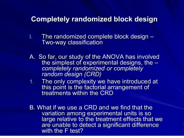
1. Randomized block designs Ó Environmental sampling and analysis (Quinn & Keough, 2002)

2. Blocking • Aim: • Reduce unexplained variation, without increasing size of experiment. • Approach: • Group experimental units (“replicates”) into blocks. • Blocks usually spatial units, one experimental unit from each treatment in each block.

3. Null hypotheses • No main effect of Factor A • H0: m1 = m2 = … = mi = ... = m • H0: a1 = a2 = … = ai = ... = 0 (ai= mi - m) • no effect of shaving domatia, pooling blocks • Factor A usually fixed

4. Null hypotheses • No effect of factor B (blocks): • no difference between blocks (leaf pairs), pooling treatments • Blocks usually random factor: • sample of blocks from populations of blocks • H0: 2 = 0

5. Randomised blocks ANOVA • Factor A with p groups (p = 2 treatments for domatia) • Factor B with q blocks (q = 14 pairs of leaves) • Source general example • Factor A p-1 1 • Factor B (blocks) q-1 13 • Residual (p-1)(q-1) 13 • Total pq-1 27

6. Randomised block ANOVA • Randomised block ANOVA is 2 factor factorial design • BUT no replicates within each cell (treatment-block combination), i.e. unreplicated 2 factor design • No measure of within-cell variation • No test for treatment by block interaction

7. Expected mean squares If factor A fixed and factor B (Blocks) random: MSAs2 + sab2 + nå(ai)2/p-1 MSBlockss2 + nsb2 MSResiduals2 + sab2

8. Residual • Cannot separately estimate s2 and sab2: • no replicates within each block-treatment combination • MSResidual estimates s2 + sab2

9. Testing null hypotheses • Factor A fixed and blocks random • If H0 no effects of factor A is true: • then F-ratio MSA / MSResidual 1 • If H0 no variance among blocks is true: • no F-ratio for test unless no interaction assumed • if blocks fixed, then F-ratio MSB / MSResidual 1

10. Assumptions • Normality of response variable • boxplots etc. • No interaction between blocks and factor A, otherwise • MSResidual increase proportionally more than MSA with reduced power of F-ratio test for A (treatments) • interpretation of main effects may be difficult, just like replicated factorial ANOVA

11. Checks for interaction • No real test because no within-cell variation measured • Tukey’s test for non-additivity: • detect some forms of interaction • Plot treatment values against block (“interaction plot”)

12. Sphericity assumption • Pattern of variances and covariances within and between “times”: • sphericity of variance-covariance matrix • Equal variances of differences between all pairs of treatments : • variance of (T1 - T2)’s = variance of (T2 - T3)’s = variance of (T1 - T3)’s etc. • If assumption not met: • F-ratio test produces too many Type I errors

13. Sphericity assumption • Applies to randomised block and repeated measures designs • Epsilon (e) statistic indicates degree to which sphericity is not met • further e is from 1, more variances of treatment differences are different • Two versions of e • Greenhouse-Geisser e • Huyhn-Feldt e

14. Dealing with non-sphericity If e not close to 1 and sphericity not met, there are 2 approaches: • Adjusted ANOVA F-tests • df for F-ratio tests from ANOVA adjusted downwards (made more conservative) depending on value e • Multivariate ANOVA (MANOVA) • treatments considered as multiple response variables in MANOVA

15. Sphericity assumption • Assumption of sphericity probably OK for randomised block designs: • treatments randomly applied to experimental units within blocks • Assumption of sphericity probably also OK for repeated measures designs: • if order each “subject” receives each treatment is randomised (eg. rats and drugs)

16. Sphericity assumption • Assumption of sphericity probably not OK for repeated measures designs involving time: • because response variable for times closer together more correlated than for times further apart • sphericity unlikely to be met • use Greenhouse-Geisser adjusted tests or MANOVA

17. Partly nested ANOVA Ó Environmental sampling and analysis (Quinn & Keough, 2002)

18. Partly nested ANOVA • Designs with 3 or more factors • Factor A and C crossed • Factor B nested within A, crossed with C

19. Partly nested ANOVA Experimental designs where a factor (B) is crossed with one factor (C) but nested within another (A). A 1 2 3 etc. B(A) 1 2 3 4 5 6 7 8 9 C 1 2 3 etc. Reps 1 2 3 n

20. ANOVA table Source df Fixed or random A (p-1) Either, usually fixed B(A) p(q-1) Random C (r-1) Either, usually fixed A * C (p-1)(r-1) Usually fixed B(A) * C p(q-1)(r-1) Random Residual pqr(n-1)

21. Linear model yijkl = m + ai + bj(i) + dk + adik + bdj(i)k + eijkl m grand mean (constant) ai effect of factor A bj(i) effect of factor B nested w/i A dk effect of factor C adik interaction b/w A and C bdj(i)k interaction b/w B(A) and C eijkl residual variation

22. Expected mean squares Factor A (p levels, fixed), factor B(A) (q levels, random), factor C (r levels, fixed) Source df EMS Test A p-1 2 + nr2 + nqr2 MSA/MSB(A) B(A) p(q-1) 2 + nr2 MSB/MSRES C r-1 2 + n2 + npq2 MSC/MSB(A)C AC (p-1)(r-1) 2 + n2 + nq2 MSAC/MSB(A)C B(A) C p(q-1)(r-1) 2 + n2 MSBC/MSRES Residual pqr(n-1) 2

23. Split-plot designs • Units of replication different for different factors • Factor A: • units of replication termed “plots” • Factor B nested within A • Factor C: • units of replication termed subplots within each plot

24. Analysis of variance • Between plots variation: • Factor A fixed - one factor ANOVA using plot means • Factor B (plots) random - nested within A (Residual 1) • Within plots variation: • Factor C fixed • Interaction A * C fixed • Interaction B(A) * C (Residual 2)

25. ANOVA Source of variation df Between plots Site 2 Plots within site (Residual 1) 3 Within plots Trampling 3 Site x trampling (interaction) 6 Plots within site x trampling (Residual 2) 9 Total 23

26. Repeated measures designs • Each whole plot measured repeatedly under different treatments and/or times • Within plots factor often time, or at least treatments applied through time • Plots termed “subjects” in repeated measures terminology

27. Repeated measures designs • Factor A: • units of replication termed “subjects” • Factor B (subjects) nested within A • Factor C: • repeated recordings on each subject

28. Repeated measures design [O2] Breathing Toad 1 2 3 4 5 6 7 8 type Lung 1 x x x x x x x x Lung 2 x x x x x x x x ... ... ... ... ... ... ... ... ... ... Lung 9 x x x x x x x x Buccal 10 x x x x x x x x Buccal 12 x x x x x x x x ... ... ... ... ... ... ... ... ... ... Buccal 21 x x x x x x x x

29. ANOVA Source of variation df Between subjects (toads) Breathing type 1 Toads within breathing type (Residual 1) 19 Within subjects (toads) [O2] 7 Breathing type x [O2] 7 Toads (Breathing type) x [O2] (Residual 2) 133 Total 167

30. Assumptions • Normality & homogeneity of variance: • affects between-plots (between-subjects) tests • boxplots, residual plots, variance vs mean plots etc. for average of within-plot (within-subjects) levels

31. No “carryover” effects: • results on one subplot do not influence results one another subplot. • time gap between successive repeated measurements long enough to allow recovery of “subject”

32. Sphericity • Sphericity of variance-covariance matrix • variances of paired differences between levels of within-plots (or subjects) factor equal within and between levels of between-plots (or subjects) factor • variance of differences between [O2] 1 and [O2] 2 = variance of differences between [O2] 2 and [O2] 2 = variance of differences between [O2] 1 and [O2] 3 etc.

33. Sphericity (compound symmetry) • OK for split-plot designs • within plot treatment levels randomly allocated to subplots • OK for repeated measures designs • if order of within subjects factor levels randomised • Not OK for repeated measures designs when within subjects factor is time • order of time cannot be randomised

34. ANOVA options • Standard univariate partly nested analysis • only valid if sphericity assumption is met • OK for most split-plot designs and some repeated measures designs

35. ANOVA options • Adjusted univariate F-tests for within-subjects factors and their interactions • conservative tests when sphericity is not met • Greenhouse-Geisser better than Huyhn-Feldt

36. ANOVA options • Multivariate (MANOVA) tests for within subjects or plots factors • responses from each subject used in MANOVA • doesn’t require sphericity • sometimes more powerful than GG adjusted univariate, sometimes not