...visualizing classifier performance in R
...visualizing classifier performance in R. Tobias Sing, Ph.D. (joint work with Oliver Sander) Modeling & Simulation Novartis Pharma AG 3 rd BaselR meeting (Oct 13, 2010). Q: When can ROCR be useful for you? Not only in machine learning!.


...visualizing classifier performance in R
E N D
Presentation Transcript
...visualizing classifier performance in R Tobias Sing, Ph.D. (joint work with Oliver Sander) Modeling & Simulation Novartis Pharma AG 3rd BaselR meeting (Oct 13, 2010)
Q: When can ROCR be useful for you?Not only in machine learning! • A: Whenever you want to evaluate a numerical score against a categorical (binary) outcome • “Does the score separate the two classes well?” 2
Examples(1) Markers of disease severity in psoriatric arthritis Numerical score: numbers of swollen and tender joints Categorical outcome: Clinical response of ACR20 improvement (yes/no) From: Englbrecht et al, 2010 3
Examples(2) HIV drug resistance • Physicians count specific mutations in the HIV genome to predict whether the virus will be resistant or susceptible to antiviral therapy. • e.g.: protease mutation list for SQV resistance from Int. AIDS Society 4
Examples(3) Evaluating scoring output from machine learning approaches • Logistic regression • model <- glm( Y ~ X, family=binomial, A) • predict(model, data.frame(X=31),type='response')[1] 0.9930342 • Decision trees • m1 <- rpart(Class ~ . ,data=GlaucomaM) • predict(m1,X)glaucoma normal0.9210526 0.078947370.1200000 0.88000000 • SVMs, Random Forests, ... 5
Scoring classifiers • Output: continuous score (instead of actual class prediction) • Example: Saquinavir (SQV) prediction with SVMs:> m <- svm(sqv[,-1], sqv[,1])> X.new <- sqv[1:2, -1]> predict(m, X.new) 1 2 TRUE TRUEUse distance to the hyperplane as numeric score:> predict(m, X.new, decision.values=TRUE)attr(,"decision.values") TRUE/FALSE1 0.99959742 0.9999517 • If predictions are (numeric) scores, actual predictions of (categorical) classes depend on the choice of a cutoff c: • f(x) ≥ c class „1“ • f(x) < c class „-1“ • Thus, a scoring classifiers induces a family {fc}c of binary classifiers
Binary classifiers (2/2)Some metrics of predictive performance • Accuracy: P(Ŷ = Y); estimated as (TP+TN) / (TP+FP+FN+TN) • Error rate: P(Ŷ ≠ Y); est: (FP+FN) / (TP+FP+FN+TN) • True positive rate (sensitivity, recall): P(Ŷ = 1 | Y = 1); est: TP / P • False positive rate (fallout): P(Ŷ = 1 | Y = -1); est: FP / N • True negative rate (specificity): P(Ŷ = -1 | Y = -1); est: FP / N • False negative rate (miss): P(Ŷ = -1 | Y = 1); est: FN / P • Precision (pos. predictive value): P(Y= 1 | Ŷ = 1); est: TP / (TP+FP) True class Predictedclass
Performance curves for visualizing trade-offs • Often the choice of a cutoff c involves trading off two competing performance measures, e.g. TPR: P(Ŷ = 1 | Y = 1) vs. FPR: P(Ŷ = 1 | Y = -1) • Performance curves (ROC, sensitivity-specificity, precision-recall, lift charts, ...) are used to visualize this trade-off
Classifier evaluation with ROCR • Only three commands • pred <- prediction( scores, labels )(pred: S4 object of class prediction) • perf <- performance( pred, measure.Y, measure.X)(pred: S4 object of class performance) • plot( perf ) • Input format • Single run:vectors (scores: numeric; labels: anything) • Multiple runs (cross-validation, bootstrapping, …): matrices or lists • Output formatFormal class 'performance' [package "ROCR"] with 6 slots| ..@ x.name : chr "Cutoff" ..@ y.name : chr "Accuracy" ..@ alpha.name : chr "none" ..@ x.values :List of 10 ..@ y.values :List of 10 ..@ alpha.values: list()
Classifier evaluation with ROCR: An example • Example: Cross-validation of saquinavir resistance prediction with SVMs> library(ROCR)Only take first training/test run for now:> pred <- prediction(as.numeric(predictions[[1]]), true.classes[[1]])> perf <- performance(pred, 'acc')> perf@y.values[[1]][1] 0.6024096 0.9397590 0.3975904You will understand in a minute why there are three accuracies (the one in the middle is relevant here) • Works exactly the same with cross-validation data (give predictions and true classes for the different folds as a list or matrix) – we have already prepared the data correctly:> str(predictions)List of 10 $ : Factor w/ 2 levels "FALSE","TRUE": 2 1 2 2 1 1 2 2 1 1 ... $ : Factor w/ 2 levels "FALSE","TRUE": 2 2 2 2 1 1 1 1 1 2 ...> pred <- prediction(lapply(predictions, as.numeric), true.classes)> perf <- performance(pred, 'acc')> perf@y.values[[1]][1] 0.6024096 0.9397590 0.3975904[[2]][1] 0.5903614 0.9638554 0.4096386
Examples (1/8): ROC curves • pred <- prediction(scores, labels) • perf <- performance(pred, "tpr", "fpr") • plot(perf, colorize=T)
Examples (2/8): Precision/recall curves • pred <- prediction(scores, labels) • perf <- performance(pred, "prec", "rec") • plot(perf, colorize=T)
Examples (3/8): Averaging across multiple runs • pred <- prediction(scores, labels) • perf <- performance(pred, "tpr", "fpr") • plot(perf, avg='threshold', spread.estimate='stddev', colorize=T)
Examples (4/8): Performance vs. cutoff • perf <- performance(pred, "cal", window.size=50) • plot(perf) • perf <- performance(pred, "acc") • plot(perf, avg= "vertical", spread.estimate="boxplot", show.spread.at= seq(0.1, 0.9, by=0.1))
Examples (5/8): Cutoff labeling • pred <- prediction(scores, labels) • perf <- performance(pred,"pcmiss","lift") • plot(perf, colorize=T, print.cutoffs.at=seq(0,1,by=0.1), text.adj=c(1.2,1.2), avg="threshold", lwd=3)
Examples (6/8): Cutoff labeling – multiple runs • plot(perf,print.cutoffs.at=seq(0,1,by=0.2),text.cex=0.8,text.y=lapply(as.list(seq(0,0.5,by=0.05)), function(x) { rep(x,length(perf@x.values[[1]]))}),col= as.list(terrain.colors(10)),text.col= as.list(terrain.colors(10)),points.col= as.list(terrain.colors(10)))
Examples (7/8): More complex trade-offs... • perf <- performance(pred,"acc","lift") • plot(perf, colorize=T) • plot(perf, colorize=T, print.cutoffs.at=seq(0,1,by=0.1), add=T, text.adj=c(1.2, 1.2), avg="threshold", lwd=3)
Examples (8/8): Some other examples • perf<-performance( pred, 'ecost') • plot(perf) • perf<-performance( pred, 'rch') • plot(perf)
Extending ROCR: An example • Extend environments • assign("auc", "Area under the ROC curve",envir = long.unit.names) • assign("auc", ".performance.auc",envir = function.names) • assign("auc", "fpr.stop", envir=optional.arguments) • assign("auc:fpr.stop", 1, envir=default.values) • Implement performance measure (predefined signature) • .performance.auc <- function (predictions, labels, cutoffs, fp, tp, fn,tn, n.pos, n.neg, n.pos.pred, n.neg.pred, fpr.stop){}
Now.... • ...get ROCR from CRAN! • demo(ROCR) [cycle through examples by hitting <Enter>, examine R code that is shown] • Help pages: • help(package=ROCR) • ?prediction • ?performance • ?plot.performance • ?'prediction-class' • ?'performance-class‘ • Please cite the ROCR paper! 21