Download

1 / 74
740 likes | 866 Views
Welcome to the Introduction to Statistics for the Social Sciences course (SBS200, COMM200, GEOG200, PA200, POL200, SOC200). In this lecture series, we will cover essential statistical concepts, including simple and multiple regression, correlation for predictions, and understanding the coefficient of determination. This course runs from Monday to Friday, from 9:00 AM to 11:20 AM, with specific locations throughout the week. Homework and reading materials will be provided online. Prepare for engaging lectures and valuable insights into statistical applications in social sciences.

E N D
. Please start your Daily Portfolio
Introduction to Statistics for the Social SciencesSBS200, COMM200, GEOG200, PA200, POL200, or SOC200Lecture Section 001, Summer Session II, 20139:00 - 11:20am Monday - FridayRoom 312 Social Sciences (Monday – Thursdays)Room 480 Marshall Building (Fridays) Welcome http://www.youtube.com/watch?v=oSQJP40PcGI
Please click in My last name starts with a letter somewhere between A. A – D B. E – L C. M – R D. S – Z Please double check All cell phones other electronic devices are turned off and stowed away
Homework due – Wednesday • On class website: • Please print and complete homework worksheet #13 • Multiple Regression
Schedule of readings Before Friday Please read chapters 10 – 14 Please read Chapters 17, and 18 in Plous Chapter 17: Social Influences Chapter 18: Group Judgments and Decisions Study Guide is online
Use this as your study guide Next couple of lectures 7/30/13 Simple and Multiple Regression Using correlation for predictions r versus r2 Regression uses the predictor variable (independent) to make predictions about the predicted variable (dependent)Coefficient of correlation is name for “r”Coefficient of determination is name for “r2”(remember it is always positive – no direction info)Standard error of the estimate is our measure of the variability of the dots around the regression line(average deviation of each data point from the regression line – like standard deviation) Coefficient of regression will “b” for each variable (like slope)
Prediction line Y’ = a+ b1X1 Frequency of Teeth brushing will be 2.77 Other Problems Y-intercept If number of cavities = 3 Slope The expected frequeny of teeth brushing for having one cavity is Frequency of teeth brushing= 5.5 + (-.91) Cavities If “Cavities” = 3, what is the prediction for “Frequency of teeth brushing”? Frequency of teeth brushing= 5.5 + (-.91) Cavities Frequency of teeth brushing= 5.5 + (-.91) (3) Frequency of teeth brushing= 5.5 + (-2.73) = 2.77 (3.0, 2.77) Review
Draw a regression line and regression equation Prediction line Y’ = b1X1+ b0 Y’ = (-.91)X 1+ 5.5 b0 = 5.5 (intercept) b1 = - 0.91(slope) r = - 0.85 Review
5 4 Number of times per day teeth are brushed 3 2 1 0 0 1 2 3 4 5 Number of cavities Correlation - let’s predict how often they brushed their teeth Find prediction line Y’ = b1 X + b0 Y’ = (-0.91) X + 5.5 Plot line - predict Y’ from X - Pick an X Let’s try X of 1 Y’ = (-0.91) 1 + 5.5 = 4.59 (plot 1,4.59) Let’s try X of 5 - Pick another X Y’ = (-0.91) 5 + 5.5 = 0.95 (plot 5,0.95) Review
5 4 Number of times per day teeth are brushed 3 2 1 0 0 1 2 3 4 5 Number of cavities X Y . 1 5 3 4 2 3 3 2 5 1 r = -0.85 b1 = - 0.91 b0 = 5.5 Y’ = b1 X + b0 Y’ = (-0.91) X + 5.5 Y’ = (-0.91) 1 + 5.5 = 4.59 Y’ = (-0.91) 3 + 5.5 = 2.77 Y’ = (-0.91) 2 + 5.5 = 3.68 Y’ = (-0.91) 3 + 5.5 = 2.77 Y’ = (-0.91) 5 + 5.5 = .95 Review
5 4 Number of times per day teeth are brushed 3 2 1 0 0 1 2 3 4 5 Number of cavities Prediction line Y’ = b1X 1+ b0 Y’ = (-.91)X 1+ 5.5 Correlation - Evaluating the prediction line Does the prediction line perfectly predict the Ys from the Xs? No, let’s see How much “error” is there? Exactly? Residuals The green lines show how much “error” there is in our prediction line…how much we are wrong in our predictions
Correlation The more closely the dots approximate a straight line,(the less spread out they are) the stronger the relationship is. Perfect correlation = +1.00 or -1.00 One variable perfectly predicts the other No variability in the scatterplot The dots approximate a straight line Any Residuals?
5 4 3 Number of times per day teeth are brushed 2 1 0 0 1 2 3 4 5 Number of cavities A note about curvilinear relationships and patterns of the residuals How well does the prediction line predict the Ys from the Xs? Residuals • Shorter green lines suggest better prediction – smaller error • Longer green lines suggest worse prediction – larger error • Why are green lines vertical? • Remember, we are predicting the variable on the Y axis • So, error would be how we are wrong about Y (vertical)
5 4 Number of times per day teeth are brushed 3 2 1 0 0 1 2 3 4 5 Number of cavities How well does the prediction line predict the Ys from the Xs? Residuals • Slope doesn’t give “variability” info • Intercept doesn’t give “variability info • Correlation “r” does give “variability info • Residuals do give “variability info
Sound familiar?? What if we want to know the “average deviation score”? Finding the standard error of the estimate (line) Standard error of the estimate (line) Standard error of the estimate: • a measure of the average amount of predictive error • the average amount that Y’ scores differ from Y scores • a mean of the lengths of the green lines
5 4 Number of times per day teeth are brushed 3 2 1 0 0 1 2 3 4 5 Number of cavities Correlation - let’s predict how often they brushed their teeth Find prediction line Y’ = b1 X + b0 Y’ = (-0.91) X + 5.5 Plot line - predict Y’ from X - Pick an X Let’s try X of 1 Y’ = (-0.91) 1 + 5.5 = 4.59 (plot 1,4.59) Let’s try X of 5 - Pick another X Y’ = (-0.91) 5 + 5.5 = 0.95 (plot 5,0.95)
X Y Y’ Y-Y’. 1 5 4.59 0.41 3 4 2.77 1.23 2 3 3.68 -0.68 3 2 2.77 -0.77 5 1 0.95 0.05 A note on Adding up deviations 5 4 Number of times per day teeth are brushed 3 2 1 0 0 1 2 3 4 5 Number of cavities r = -0.85 b1 = - 0.91 b0 = 5.5 .41 Y’ = b1 X + b0 Y’ = (-0.91) X + 5.5 1.23 -.68 Y’ = (-0.91) 1 + 5.5 = 4.59 0.05 -.77 Y’ = (-0.91) 3 + 5.5 = 2.77 Y’ = (-0.91) 2 + 5.5 = 3.68 Y’ = (-0.91) 4+ 5.5 = 1.86 Y’ = (-0.91) 5 + 5.5 = .95 These are our “predicted values” for each X score
X Y Y’ Y-Y’. (Y-Y’)2 1 5 4.59 0.41 0.168 3 4 2.77 1.23 1.513 2 3 3.68 -0.68 0.462 3 2 2.77 -0.77 0.593 5 1 0.95 0.05 .0025 5 4 Number of times per day teeth are brushed 3 2 1 0 0 1 2 3 4 5 Number of cavities r = -0.85 b1 = - 0.91 b0 = 5.5 2.739 .41 Y’ = b1 X + b0 Y’ = (-0.91) X + 5.5 1.23 -.68 Y’ = (-0.91) 1 + 5.5 = 4.59 0.05 -.77 Y’ = (-0.91) 3 + 5.5 = 2.77 Y’ = (-0.91) 2 + 5.5 = 3.68 Y’ = (-0.91) 4+ 5.5 = 1.86 Y’ = (-0.91) 5 + 5.5 = .95 This is like our average (or standard) size of our residual 2.739 0.95 “Standard Error of the Estimate” 3
Which minimizes errorbetter? 5 4 Number of times per day teeth are brushed 3 2 1 0 0 1 2 3 4 5 Number of cavities Is the regression line better than just guessing the mean of the Y variable?How much does the information about the relationship actually help? 5 4 # of times teeth are brushed 3 2 1 0 0 1 2 3 4 5 Number of cavities How much better does the regression line predict the observed results? r2 Wow!
What is r2? r2 = The proportion of the total variance in one variable that is predictable by its relationship with the other variable Examples If mother’s and daughter’s heights are correlated with an r = .8, then what amount (proportion or percentage) of variance of mother’s height is accounted for by daughter’s height? .64 because (.8)2 = .64
What is r2? r2 = The proportion of the total variance in one variable that is predictable for its relationship with the other variable Examples If mother’s and daughter’s heights are correlated with an r = .8, then what proportion of variance of mother’s height is not accountedfor by daughter’s height? .36 because (1.0 - .64) = .36 or 36% because 100% - 64% = 36%
What is r2? r2 = The proportion of the total variance in one variable that is predictable for its relationship with the other variable Examples If ice cream sales and temperature are correlated with an r = .5, then what amount (proportion or percentage) of variance of ice cream sales is accounted for by temperature? .25 because (.5)2 = .25
What is r2? r2 = The proportion of the total variance in one variable that is predictable for its relationship with the other variable Examples If ice cream sales and temperature are correlated with an r = .5, then what amount (proportion or percentage) of variance of ice cream sales is not accountedfor by temperature? .75 because (1.0 - .25) = .75 or 75% because 100% - 25% = 75%
regression equations Questions on homework?
+0.92 positive strong The relationship between the hours worked and weekly pay is a strong positive correlation. This correlation is significant, r(3) = 0.92; p < 0.05 up down 55.286 6.0857 y' = 6.0857x + 55.286 207.43 85.71 .846231 or 84% 84% of the total variance of “weekly pay” is accounted for by “hours worked” For each additional hour worked, weekly pay will increase by $6.09
400 380 360 Wait Time 340 320 300 280 7 8 6 5 4 Number of Operators
Critical r = 0.878 No we do not reject the null -.73 negative strong The relationship between wait time and number of operators working is negative and strong. This correlation is not significant, r(3) = 0.73; n.s. number of operators increase, wait time decreases 458 -18.5 y' = -18.5x + 458 365 seconds 328 seconds .53695 or 54% The proportion of total variance of wait time accounted for by number of operators is 54%. For each additional operator added, wait time will decrease by 18.5 seconds
39 36 33 30 27 24 21 Percent of BAs 45 48 51 54 57 60 63 66 Median Income
Critical r = 0.632 Yes we reject the null Percent of residents with a BA degree 10 8 0.8875 positive strong The relationship between median income and percent of residents with BA degree is strong and positive. This correlation is significant, r(8) = 0.89; p < 0.05. median income goes up so does percent of residents who have a BA degree 3.1819 0.0005 y' = 0.0005x + 3.1819 25% of residents 35% of residents .78766 or 78% The proportion of total variance of % of BAs accounted for by median income is 78%. For each additional $1 in income, percent of BAs increases by .0005
30 27 24 21 18 15 12 Crime Rate 45 48 51 54 57 60 63 66 Median Income
Critical r = 0.632 No we do not reject the null Crime Rate 10 8 -0.6293 negative moderate The relationship between crime rate and median income is negative and moderate. This correlation is not significant, r(8) = -0.63; p < n.s. [0.6293 is not bigger than critical of 0.632] . median income goes up, crime rate tends to go down 4662.5 -0.0499 y' = -0.0499x + 4662.5 2,417 thefts 1,418.5 thefts .396 or 40% The proportion of total variance of thefts accounted for by median income is 40%. For each additional $1 in income, thefts go down by .0499
Example of Simple Regression The manager of copier company wants to determine whether there is a relationship between the number of sales calls made in a month and the number of copiers sold that month. The manager selects a random sample of 10 representatives and determines the number of sales calls each representative made last month and the number of copiers sold.
Correlation: Independent and dependent variables • When used for prediction we refer to the predicted variable • as the dependent variable and the predictor variable as the independent variable What are we predicting? Who sold the most copiers? Who sold the fewest copiers? Soni Carlos Jeff Mark Susan Tom Dependent Variable Independent Variable
Correlation Coefficient– Excel Example • Interpret r = 0.759 • Positive relationship between the number of sales calls and the number of copiers sold. • Strong relationship • Remember, we have not demonstrated cause and effect here, only that the two variables—sales calls and copiers sold—are related. 0.759014
Correlation Coefficient– Excel Example • Interpret r = 0.759 • Does this correlation reach significance? • n = 10, df = 8 • alpha = .05 • Observed r is larger than critical r (0.759 > 0.632) therefore we reject the null hypothesis. • r (8) = 0.759; p < 0.05 0.759014
Coefficient of Determination– Excel Example • Interpret r2 = 0.576(.7592 = .576) • we can say that 57.6 percent of the variation in the number of copiers sold is explained, or accounted for, by the variation in the number of sales calls. • Remember, we lose the directionality of the relationship with the r2 0.759014
Regression Equation- Example If you probably sell this much State the regression equation Y’ = a + bx Y’ = 18.9476 + 1.1842x If make this many calls Interpret the slope Y’ = 18.9476 + 1.1842x “For each additional sales call made we sell 1.842 more copiers” Solve for some value of Y’ Y’ = 18.9476 + 1.1842 (20) Y’ = 42.63 What is the expected number of copiers sold by a representative who made 20 calls?
Regression Equation- Example If you probably sell this much If make this many calls Solve for some value of Y’ Y’ = 18.9476 + 1.1842 (40) Y’ = 66.3156 What is the expected number of copiers sold by a representative who made 40 calls?
An example for The Standard Error of Estimate The standard error of estimate measures the scatter, or dispersion, of the observed values around the line of regression A formula that can be used to compute the standard error: Standard error of the estimate (line)
Regression Analysis – Least Squares Principle When we calculate the regression line we try to: • minimize distance between predicted Ys and actual (data) Y points (length of green lines) • remember because of the negative and positive values cancelling each other out we have to square those distance (deviations) • so we are trying to minimize the “sum of squares of the vertical distances between the actual Y values and the predicted Y values”
The Standard Error of Estimate Step 1: List all the Y data points
The Standard Error of Estimate Step 1: List all the Y data points Step 2: Find all the predicted Y’ data points
The Standard Error of Estimate Step 3: Find deviations Step 4: Square and add up deviations
Then simply plug in the numbers and solve for the standard error of the estimate Remember conceptually, this is like the average of the length of those green lines 784.211 = = 9.901 10 - 2
Writing Assignment - 5 Questions 1. What is regression used for? • Include and example 2. What is a residual? How would you find it? 3. What is Standard Error of the Estimate (How is it related to residuals?) 4. Give one fact about r2 5. How is regression line like a mean?
Writing Assignment - 5 Questions 1. What is regression used for? • Include and example Regressions are used to take advantage of relationships between variables described in correlations. We choose a value on the independent variable (on x axis) to predict values for the dependent variable (on y axis).