Support Vector Machine & Its Applications
Support Vector Machine & Its Applications. Mingyue Tan The University of British Columbia Nov 26, 2004. A portion (1/3) of the slides are taken from Prof. Andrew Moore’s SVM tutorial at http://www.cs.cmu.edu/~awm/tutorials. Overview.

Support Vector Machine & Its Applications
E N D
Presentation Transcript
Support Vector Machine & Its Applications Mingyue Tan The University of British Columbia Nov 26, 2004 A portion (1/3) of the slides are taken from Prof. Andrew Moore’s SVM tutorial at http://www.cs.cmu.edu/~awm/tutorials
Overview • Intro. to Support Vector Machines (SVM) • Properties of SVM • Applications • Gene Expression Data Classification • Text Categorization if time permits • Discussion
a Linear Classifiers x f yest f(x,w,b) = sign(w x+ b) denotes +1 denotes -1 w x+ b>0 w x+ b=0 How would you classify this data? w x+ b<0
a Linear Classifiers x f yest f(x,w,b) = sign(w x +b) denotes +1 denotes -1 How would you classify this data?
a Linear Classifiers x f yest f(x,w,b) = sign(w x+ b) denotes +1 denotes -1 How would you classify this data?
a Linear Classifiers x f yest f(x,w,b) = sign(w x+ b) denotes +1 denotes -1 Any of these would be fine.. ..but which is best?
a Linear Classifiers x f yest f(x,w,b) = sign(w x +b) denotes +1 denotes -1 How would you classify this data? Misclassified to +1 class
a a Classifier Margin Classifier Margin x x f f yest yest f(x,w,b) = sign(w x +b) f(x,w,b) = sign(w x +b) denotes +1 denotes -1 denotes +1 denotes -1 Define the margin of a linear classifier as the width that the boundary could be increased by before hitting a datapoint. Define the margin of a linear classifier as the width that the boundary could be increased by before hitting a datapoint.
a Maximum Margin x f yest • Maximizing the margin is good according to intuition and PAC theory • Implies that only support vectors are important; other training examples are ignorable. • Empirically it works very very well. f(x,w,b) = sign(w x+ b) denotes +1 denotes -1 The maximum margin linear classifier is the linear classifier with the, um, maximum margin. This is the simplest kind of SVM (Called an LSVM) Support Vectors are those datapoints that the margin pushes up against Linear SVM
Linear SVM Mathematically x+ M=Margin Width “Predict Class = +1” zone What we know: • w . x+ + b = +1 • w . x- + b = -1 • w . (x+-x-) = 2 X- wx+b=1 “Predict Class = -1” zone wx+b=0 wx+b=-1
Linear SVM Mathematically • Goal: 1) Correctly classify all training data if yi = +1 if yi = -1 for all i 2) Maximize the Margin same as minimize • We can formulate a Quadratic Optimization Problem and solve for w and b • Minimize subject to
Solving the Optimization Problem Find w and b such that Φ(w) =½ wTw is minimized; and for all {(xi,yi)}: yi (wTxi+ b)≥ 1 • Need to optimize a quadratic function subject to linear constraints. • Quadratic optimization problems are a well-known class of mathematical programming problems, and many (rather intricate) algorithms exist for solving them. • The solution involves constructing a dual problem where a Lagrange multiplierαi is associated with every constraint in the primary problem: Find α1…αNsuch that Q(α) =Σαi- ½ΣΣαiαjyiyjxiTxjis maximized and (1)Σαiyi= 0 (2) αi≥ 0 for all αi
The Optimization Problem Solution • The solution has the form: • Each non-zero αi indicates that corresponding xi is a support vector. • Then the classifying function will have the form: • Notice that it relies on an inner product between the test point xand the support vectors xi– we will return to this later. • Also keep in mind that solving the optimization problem involved computing the inner products xiTxj between all pairs of training points. w =Σαiyixi b= yk- wTxkfor any xksuch that αk 0 f(x) = ΣαiyixiTx + b
denotes +1 denotes -1 Dataset with noise • Hard Margin: So far we require all data points be classified correctly - No training error • What if the training set is noisy? - Solution 1: use very powerful kernels OVERFITTING!
e11 e2 wx+b=1 e7 wx+b=0 wx+b=-1 Soft Margin Classification Slack variablesξi can be added to allow misclassification of difficult or noisy examples. What should our quadratic optimization criterion be? Minimize
Hard Margin v.s. Soft Margin • The old formulation: • The new formulation incorporating slack variables: • Parameter C can be viewed as a way to control overfitting. Find w and b such that Φ(w) =½ wTw is minimized and for all {(xi,yi)} yi (wTxi+ b)≥ 1 Find w and b such that Φ(w) =½ wTw + CΣξi is minimized and for all {(xi,yi)} yi(wTxi+ b)≥ 1- ξi and ξi≥ 0 for all i
Linear SVMs: Overview • The classifier is a separating hyperplane. • Most “important” training points are support vectors; they define the hyperplane. • Quadratic optimization algorithms can identify which training points xi are support vectors with non-zero Lagrangian multipliers αi. • Both in the dual formulation of the problem and in the solution training points appear only inside dot products: Find α1…αNsuch that Q(α) =Σαi- ½ΣΣαiαjyiyjxiTxj is maximized and (1) Σαiyi= 0 (2) 0 ≤αi≤ C for all αi f(x) = ΣαiyixiTx + b
x 0 x 0 x2 Non-linear SVMs • Datasets that are linearly separable with some noise work out great: • But what are we going to do if the dataset is just too hard? • How about… mapping data to a higher-dimensional space: 0 x
Non-linear SVMs: Feature spaces • General idea: the original input space can always be mapped to some higher-dimensional feature space where the training set is separable: Φ: x→φ(x)
The “Kernel Trick” • The linear classifier relies on dot product between vectors K(xi,xj)=xiTxj • If every data point is mapped into high-dimensional space via some transformation Φ: x→ φ(x), the dot product becomes: K(xi,xj)= φ(xi)Tφ(xj) • A kernel function is some function that corresponds to an inner product in some expanded feature space. • Example: 2-dimensional vectors x=[x1 x2]; let K(xi,xj)=(1 + xiTxj)2, Need to show that K(xi,xj)= φ(xi)Tφ(xj): K(xi,xj)=(1 + xiTxj)2, = 1+ xi12xj12 + 2 xi1xj1xi2xj2+ xi22xj22 + 2xi1xj1 + 2xi2xj2 = [1 xi12 √2 xi1xi2 xi22 √2xi1 √2xi2]T [1 xj12 √2 xj1xj2 xj22 √2xj1 √2xj2] = φ(xi)Tφ(xj), where φ(x) = [1 x12 √2 x1x2 x22 √2x1 √2x2]
What Functions are Kernels? • For some functions K(xi,xj) checking that K(xi,xj)= φ(xi)Tφ(xj) can be cumbersome. • Mercer’s theorem: Every semi-positive definite symmetric function is a kernel • Semi-positive definite symmetric functions correspond to a semi-positive definite symmetric Gram matrix: K=
Examples of Kernel Functions • Linear: K(xi,xj)= xi Txj • Polynomial of power p: K(xi,xj)= (1+xi Txj)p • Gaussian (radial-basis function network): • Sigmoid: K(xi,xj)= tanh(β0xi Txj + β1)
Non-linear SVMs Mathematically • Dual problem formulation: • The solution is: • Optimization techniques for finding αi’s remain the same! Find α1…αNsuch that Q(α) =Σαi- ½ΣΣαiαjyiyjK(xi,xj) is maximized and (1) Σαiyi= 0 (2) αi≥ 0 for all αi f(x) = ΣαiyiK(xi,xj)+ b
Nonlinear SVM - Overview • SVM locates a separating hyperplane in the feature space and classify points in that space • It does not need to represent the space explicitly, simply by defining a kernel function • The kernel function plays the role of the dot product in the feature space.
Properties of SVM • Flexibility in choosing a similarity function • Sparseness of solution when dealing with large data sets - only support vectors are used to specify the separating hyperplane • Ability to handle large feature spaces - complexity does not depend on the dimensionality of the feature space • Overfitting can be controlled by soft margin approach • Nice math property: a simple convex optimization problem which is guaranteed to converge to a single global solution • Feature Selection
SVM Applications • SVM has been used successfully in many real-world problems - text (and hypertext) categorization - image classification - bioinformatics (Protein classification, Cancer classification) - hand-written character recognition
Application 1: Cancer Classification • High Dimensional - p>1000; n<100 • Imbalanced - less positive samples • Many irrelevant features • Noisy FEATURE SELECTION In the linear case, wi2 gives the ranking of dim i SVM is sensitive to noisy (mis-labeled) data
Weakness of SVM • It is sensitive to noise - A relatively small number of mislabeled examples can dramatically decrease the performance • It only considers two classes - how to do multi-class classification with SVM? - Answer: 1) with output arity m, learn m SVM’s • SVM 1 learns “Output==1” vs “Output != 1” • SVM 2 learns “Output==2” vs “Output != 2” • : • SVM m learns “Output==m” vs “Output != m” 2)To predict the output for a new input, just predict with each SVM and find out which one puts the prediction the furthest into the positive region.
Application 2: Text Categorization • Task: The classification of natural text (or hypertext) documents into a fixed number of predefined categories based on their content. - email filtering, web searching, sorting documents by topic, etc.. • A document can be assigned to more than one category, so this can be viewed as a series of binary classification problems, one for each category
Representation of Text IR’s vector space model (aka bag-of-words representation) • A doc is represented by a vector indexed by a pre-fixed set or dictionary of terms • Values of an entry can be binary or weights • Normalization, stop words, word stems • Doc x => φ(x)
Text Categorization using SVM • The distance between two documents is φ(x)·φ(z) • K(x,z) = 〈φ(x)·φ(z) is a valid kernel, SVM can be used with K(x,z) for discrimination. • Why SVM? -High dimensional input space -Few irrelevant features (dense concept) -Sparse document vectors (sparse instances) -Text categorization problems are linearly separable
Some Issues • Choice of kernel - Gaussian or polynomial kernel is default - if ineffective, more elaborate kernels are needed - domain experts can give assistance in formulating appropriate similarity measures • Choice of kernel parameters - e.g. σ in Gaussian kernel - σ is the distance between closest points with different classifications - In the absence of reliable criteria, applications rely on the use of a validation set or cross-validation to set such parameters. • Optimization criterion – Hard margin v.s. Soft margin - a lengthy series of experiments in which various parameters are tested
Additional Resources • An excellent tutorial on VC-dimension and Support Vector Machines: C.J.C. Burges. A tutorial on support vector machines for pattern recognition. Data Mining and Knowledge Discovery, 2(2):955-974, 1998. • The VC/SRM/SVM Bible: Statistical Learning Theory by Vladimir Vapnik, Wiley-Interscience; 1998 http://www.kernel-machines.org/
Reference • Support Vector Machine Classification of Microarray Gene Expression Data, Michael P. S. Brown William Noble Grundy, David Lin, Nello Cristianini, Charles Sugnet, Manuel Ares, Jr., David Haussler • www.cs.utexas.edu/users/mooney/cs391L/svm.ppt • Text categorization with Support Vector Machines:learning with many relevant features T. Joachims, ECML - 98