Image Analysis and Classification
Image Analysis and Classification. Padhraic Smyth Information and Computer Science CS 175, Fall 2007. Multiple 3d interpretations are possible for a 2d image due to visual ambiguity. One Interpretation. Another Interpretation. Sources of Variation in Intensity Images.


Image Analysis and Classification
E N D
Presentation Transcript
Image Analysis and Classification Padhraic Smyth Information and Computer Science CS 175, Fall 2007
Multiple 3d interpretations are possible for a 2d image due to visual ambiguity
Sources of Variation in Intensity Images • Assume we are looking at a specific object (e.g., a face) • Assume the light source, camera, etc., are fixed • There are two systematic sources of variation: • Object-specific variation • variations in reflectance • bright skin, dark hair, lips • shadows • nose, mouth, ears • texture variation • curly hair versus flat hair, etc • Viewpoint-specific variation (next slide)
Viewpoint-specific Variation • This is the variation in the intensity values which arises from changes in the relative position of the camera and the face • it is not an “intrinsic property” of the face • so it typically gets in the way of recognition, classification • Scale: • distance of the face to the camera • Translation • relative position of the face in the image • e.g., centered or not • Orientation/Pose • angle of the face relative to the image • e.g., looking upwards or sideways • Deformation • the face is distorted from its “normal” position • smiling, shouting, etc
Variations in face images • Consider an image of the face of George Bush • what are all the variations one could have in images of his face? • short-term variations: • scale(distance) • translation (position in image) • orientation (pose) • expression • lighting (day, night, shadows) • sunglasses • hair-style • longer-term variations • “weight” • beard, moustache • scar/injury
Recognizing George Bush’s face • Images from Google Image Search • Note variations in • scale • face orientation • lighting • scene complexity, etc
Image Classification • Say we want to build a system which outputs a 1 when George Bush is in the picture and a 0 otherwise • This is a classification problem: • 2 classes: • Class 1: “image contains George Bush” • Class 2: “image does not contain George Bush” • What could we use as features (the inputs to the classifier)? • The M x N pixels in each image (if all images are the same size) • Or we could use features derived from the image • location, size of face • relative position of eyes from nose, etc • this assumes we can find the face in the image
Stages in Face Classification Face Locator INTENSITY IMAGE Feature Extraction Classifier Classification Decision
Stages in Face Classification • Face Location: • find the set of pixels that look most like a face • What do if there are multiple faces? No faces? • Becomes harder as there is more variation in appearance (orientation, scale, etc) • For certain images (e.g., “mug shots”) we could use all pixels in the image and skip the step of locating the face • Feature Extraction • extract specific features for each region of interest (high-level) • e.g., shape of object, size of nose, relative position of eyes,etc • an alternative is to use the pixels directly as features (low-level) • Classification: • classify features into “face” or “not a face” • classifier is trained on training data • positive examples: images with the desired faces • negative examples: images without the desired faces
Different types of Face Classification • Identification • Class i = ith person in the database, i goes from 1 to M • Class M+1 = everyone else • Binary version of Identification • Class 1 = “is in the database” (e.g., is an employee) • Class 2 = “is not in the database” (e.g., is not an employee) • Detection • class 1 = there is at least 1 face in the image • class 2 = there is no face in the image • Classification of face types • class 1 = male face, class 2 = female face • class 1 = has a beard, class 2 = does not have a beard
Applications of Face Recognition • Security • automatic identification of a user for building entry, airport security • Retrieval and Annotation • news services have large databases of video/image data • would like to quickly be able to find “images of Bill Clinton with Gov. Arnold” • Online photo databases (e.g., Flickr) • Automatically annotate images (e.g., do they have faces or not?) • User Interfaces • recognition of user at terminal, personalized interface • recognition of human emotions • Handicapped Services • automated “lip-reading”, recognition of faces for blind people
Recognizing George Bush’s face • Images from Google Image Search • Note variations in • scale • face orientation • lighting • scene complexity, etc
Locating any Face in an Image • Images from Google Image Search • Note variations in • scale • face orientation • lighting • scene complexity, etc
Which images contain human faces? Images from New York Times Web page, Note variety of types of images, lighting, scale, orientation
perceptron.m function function [outputs] = perceptron(weights,data) % function [outputs] = perceptron(weights,data) % % Compute the class predictions for perceptron (linear classifier) % Sample code for CS 175 % % Inputs % weights: 1 x (d+1) row vector of weights % data: N x (d+1) matrix of training data % % Outputs % outputs: N x 1 vector of perceptron outputs % error checking if size(weights,1) ~= 1 error('The first argument (weights) should be a row vector'); end if size(data,2) ~= size(weights,2) error('The arguments (weights and data) should have the same number of columns'); end % calculate the thresholded outputs of the perceptron (vectorized) outputs = sign(data*weights');
perceptron_error.m function function [cerror, mse] = perceptron_error(weights,data,targets) % function [cerror, mse] = perceptron_error(weights,data,targets) % % Compute mis-classification error and mean squared error for % a perceptron (linear) classifier % Sample code for CS 175 % % Inputs % weights: 1 x (d+1) row vector of weights % data: N x (d+1) matrix of training data % targets: N x 1 vector of target values (+1 or -1) % % Outputs % cerror: the percentage of examples misclassified (between 0 and 100) % mse: the mean-square error (sum of squared errors divided by N)
perceptron_error.m function N = size(data, 1); % error checking if nargin ~= 3 error('The function takes three arguments (weights, data, targets)'); end if size(weights,1) ~= 1 error('The first argument (weights) should be a row vector'); end if size(data,2) ~= size(weights,2) error('The first two arguments (weights and data) should have the same number of columns'); end if size(data,1) ~= size(targets,1) error('The last two arguments (targets and data) should have the same number of rows'); end
perceptron_error.m function % calculate the unthresholded outputs, for all rows in data, N x 1 vector f = (weights * data‘) ‘; % compare thresholded output to the target values to get the accuracy cerror = 100 * sum(sign(f) ~= targets)/N; % calculate the sigmoid version of the outputs, for all rows in data, N x 1 vector outputs = sigmoid(f); % compare sigmoid output vector to the target vector to get the mse mse = sum((outputs-targets).^2)/N; function s = sigmoid(x) % Computes sigmoid function (scaled to -1, +1) s = 2./(1+exp(-x)) - 1;
perceptron_error.m function % calculate the unthresholded outputs, for all rows in data, N x 1 vector f = (weights * data‘) ‘; % compare thresholded output to the target values to get the accuracy cerror = 100 * sum(sign(f) ~= targets)/N; % calculate the sigmoid version of the outputs, for all rows in data, N x 1 vector outputs = sigmoid(f); % compare sigmoid output vector to the target vector to get the mse mse = sum((outputs-targets).^2)/N; function s = sigmoid(x) % Computes sigmoid function (scaled to -1, +1) s = 2./(1+exp(-x)) - 1; Vectorized computation of classification error rate Vectorized computation of sigmoid output Vectorized computation of MSE Local function defining the sigmoid. Note that it works on vectors
Principle of Gradient Descent Gradient descent algorithm: • Start with some initial guess at w • Move downhill in “small steps” direction of steepest descent • What is the direction of steepest descent? • The negative of the gradient, evaluated at w • What is the gradient? • Gradient = vector of derivatives with respect to each component of w • E.g., if w = [ w1, w2, w3] then gradient[g(w)] = [ d g(w)/ dw1, d g(w)/dw2, d g(w)/dw3 ] • Note that the gradient is itself a vector (or a “direction) • After moving, recompute the gradient, get a new downhill direction, and move again. • Keep repeating this until the decrease in g(w) is less than some threshold, i.e., we appear to be on a flat part of the g(w) surface.
Illustration of Gradient Descent g(w) w1 w2
Illustration of Gradient Descent g(w) w1 w2
Illustration of Gradient Descent g(w) w1 Direction of steepest descent = direction of negative gradient w2
Illustration of Gradient Descent g(w) w1 Original point in weight space New point in weight space w2
Gradient Descent Algorithm • Algorithm converges to either • Global minimum if g(w) is convex (has a single minimum) • this is the case for the perceptron • Local minimum if g(w) has multiple local minima • This is the case for multilayer neural networks • To avoid local minima, in practice we rerun the gradient descent algorithm from multiple random starting points pick the solution with the lowest MSE. • Note that the backpropagation algorithm is based on gradient descent (using a clever way to calculate the gradient) • Note that the algorithm need not converge at all if the learning rate (i.e., step size) is too large
Gradient Descent Algorithm Mathematically, the Gradient Descent Rule: wnew = wold - h D (w) where D (w) is the gradient and h is the learning rate (small, positive)
Gradient Descent Algorithm Mathematically, the Gradient Descent Rule: wnew = wold - h D (w) where D (w) is the gradient and h is the learning rate (small, positive) In MATLAB, for the perceptron with sigmoid outputs this translates into the following update rule: weights = weights - rate * (o - targets(i)) * dsigmoid(o) * data(i, :); This whole part is the gradient, evaluated at the current weight vector
learn_perceptron.m function function [weights,mse,acc] = learn_perceptron(data,targets,rate,threshold,init_method,random_seed,plotflag,k) % function [weights,mse,acc] = learn_perceptron(data,targets,rate,threshold,init_method,random_seed,plotflag,k) % % Learn the weights for a perceptron (linear) classifier to minimize its % mean squared error. % Sample code for CS 175 % % Inputs % data: N x (d+1) matrix of training data % targets: N x 1 vector of target values (+1 or -1) % rate: learning rate for the perceptron algorithm (e.g., rate = 0.001) % threshold: if the reduction in MSE from one iteration to the next is *less* % than threshold, then halt learning (e.g., threshold = 0.000001) % init_method: method used to initialize the weights (1 = random, 2 = half % way between 2 random points in each group, 3 = half way between % the centroids in each group) % random_seed: this is an integer used to "seed" the random number generator % for either methods 1 or 2 for initialization (this is useful % to be able to recreate a particular run exactly) % plotflag: 1 means plotting is turned on, default value is 0 % k: how many iterations between plotting (e.g., k = 100) % % Outputs % weights: 1 x (d+1) row vector of learned weights % mse: mean squared error for learned weights % acc: classification accuracy for learned weights (percentage, between 0 and 100)
learn_perceptron.m function [N, d] = size(data); % error checking if nargin < 4 error('The function takes at least 4 arguments (data, targets, rate, threshold)'); end if size(data,1) ~= size(targets,1) error('The number of rows in the first two arguments (data, targets) does not match!'); end % initialize the input arguments if ~exist('k') k = 100; end if ~exist('plotflag') plotflag = 0; end if ~exist('random_seed') random_seed = 1234; end if ~exist('init_method') init_method = 1; end
learn_perceptron.m function % initialize the weights weights = initialize_weights175(data,targets,init_method,random_seed); iteration=0; while iteration < 2 | ( abs(mse(iteration) - mse(iteration-1)) > threshold ) iteration = iteration + 1; % cycle through all of the examples for i=1:N % calculate the unthresholded output for the ith row of "data" o = sigmoid( weights * data(i,:)' ); % update the weight vector weights = weights + rate * (targets(i) - o) * dsigmoid(o) * data(i, :); end % calculate the errors using current parameter values [cerror(iteration), mse(iteration)] = perceptron_error(weights, data, targets); % visualize the decision boundary if needed if plotflag == 1 & mod(iteration - 1, k) == 0 t = strcat ('Decision boundary at iteration # ', num2str(iteration)); weightplot175(data, targets, weights, t); pause(0.0001); end end
learn_perceptron.m function % create the plots of the MSE and Accuracy Vs. iteration number if (plotflag == 1) figure(2); subplot(2, 1, 1); plot(mse,'b-'); xlabel('iteration'); ylabel('MSE'); subplot(2, 1, 2); plot(100-cerror,'b-'); xlabel('iteration'); ylabel('Accuracy'); end % local functions….. function s = sigmoid(x) % Compute the sigmoid function, scaled from -1 to +1 s = 2./(1+exp(-x)) - 1; function ds = dsigmoid(x) % Compute the derivative of the (rescaled) sigmoid ds = .5 .* (sigmoid(x)+1) .* (1-sigmoid(x));
Demonstration script % CS 175 demo script to illustrate perceptron learning..... load sampledata2 data2 = [data2 ones(40,1)]; pause help initialize_weights175 w = initialize_weights175(data2,targets2,2,1234); whos pause help weightplot175 weightplot175(data2,targets2,w,'initial weights'); pause help learn_perceptron [weights,mse,acc] = learn_perceptron(data2,targets2,0.001,0.00001,2,1234,1,50); pause [weights,mse,acc] = learn_perceptron(data2,targets2,0.001,0.00001,1,123,1,200); pause [weights,mse,acc] = learn_perceptron(data2,targets2,0.001,0.000001,1,123,1,500); pause
Illustration of perceptron with images % script to illustrate learning of image classifiers using perceptrons load imagedata; % imagedata.mat from Assignment 4 umatrix = image_to_matrix(uimages); rmatrix = image_to_matrix(rimages); smatrix = image_to_matrix(simages); % create a 2-class data set for right images and straight images data = [rmatrix ones(20,1); smatrix ones(18,1)]; targets = [ones(20,1);ones(18,1)*(-1)]; % run the perceptron.... [weights,mse,acc] = learn_perceptron(data,targets,0.001,0.000001,2,1234,0,50); % should get these results: % Hit any key to start perceptron learning.....
Illustration of perceptron with images [weights,mse,acc] = learn_perceptron(data,targets,0.001,0.000001,2,1234,0,50); % should get these results: % Hit any key to start perceptron learning..... % % Iteration 1: accuracy = 50.000, MSE = 1.927847 % Iteration 51: accuracy = 55.263, MSE = 1.728016 % Iteration 101: accuracy = 65.789, MSE = 1.285193 % Iteration 151: accuracy = 76.316, MSE = 0.996258 % Iteration 201: accuracy = 76.316, MSE = 0.717544 % Iteration 251: accuracy = 89.474, MSE = 0.328408 % Iteration 301: accuracy = 92.105, MSE = 0.308942 % % % Hit any key to display the final results..... % Final results: % Iteration 326: accuracy = 89.474, MSE = 0.309101 size(weights) % ans = % 1 961 % look at the weights as an image.... x = reshape(weights(1:960),30,32); dispimg(x)
MATLAB code to look at mean and difference images load imagedata; % imagedata.mat from Assignment 4 umatrix = image_to_matrix(uimages); rmatrix = image_to_matrix(rimages); smatrix = image_to_matrix(simages); % generate the mean image for each group: mean_uimage = reshape(mean(umatrix),30,32); mean_simage = reshape(mean(smatrix),30,32); mean_rimage = reshape(mean(rmatrix),30,32);
image_to_matrix function function matrix = image_to_matrix(imageset) % function matrix = image_to_matrix(imageset) % % INPUT: % imageset: m by n structure array where imageset(i,j).image is a matrix of pixel (image) % values of size x by y % % OUTPUT: % matrix: a m*n (number of images) by x*y (pixels per image) array of images in vector % form, where each row is one image [m n] = size(imageset); N = m * n; idx = 0; for i = 1:N % skip empty images if idx == 0 & size(imageset(i).image) ~= [1,1] % get the dimensions of the non-empty image [nx, ny] = size(imageset(i).image); idx = 1; end if size(imageset(i).image) == [nx,ny] % convert into a vector matrix(idx,:) = reshape(imageset(i).image,1,nx*ny); idx = idx + 1; end end if ~exist('matrix') error('Imageset contains empty images only!'); end
MATLAB code to look at mean and difference images % note below: to get dispimg.m to work with subplots, need to comment out % the "figure" command within dispimg figure(1); subplot(2,2,1);dispimg(mean_simage); title('Mean of Straight Images'); subplot(2,2,3);dispimg(mean_uimage); title('Mean of Up Images'); subplot(2,2,2);dispimg(mean_simage - mean_uimage); title('Mean Difference Image'); figure(2); subplot(2,2,1);dispimg(mean_simage); title('Mean of Straight Images'); subplot(2,2,3);dispimg(mean_rimage); title('Mean of Right Images'); subplot(2,2,2);dispimg(mean_simage - mean_rimage); title('Mean Difference Image');
Additional Concepts in Classification (useful for Assignment 4)
The Minimum-Distance Classifier • A very simple classifier • Assume we have data from M classes (e.g., M=2) • Calculate the mean for each class, e.g., Mean1 and Mean2 • mean vector = sum of all vectors/number of vectors • mean vector ~ “centroid” of points • Classify each new point x as follows • for j = 1: M • calculate the distance dj = Euclidean distance(x, Meanj) • distance from x to the jth “class mean” • choose the minimum distance as the predicted class • assign x to the closest mean
Assignment 4: Minimum Distance Classifier (provided) function acc = minimum_distance(traindata,trainlabels,testdata,testlabels) % % implementation of a minimum distance classifier % % INPUTS: % traindata: N1 x d matrix of feature data % trainlabels: N1 x 1 column vector of classlabels % testdata: N2 x d matrix of feature data % trainlabels: N2 x 1 column vector of classlabels % % OUTPUTS: % acc: accuracy (percentage) on the test data for a classifier % trained on the training data