Lidar for Basemaps:
320 likes | 498 Views
Lidar for Basemaps:. Getting the Most From Your Data. Eddie Bergeron, SVO June 29, 2010. Lidar Basics Review. An aircraft flies over the terrain sending out laser pulses, counting the time it takes for the pulse reflections to bounce off of objects and return

Lidar for Basemaps:
E N D
Presentation Transcript
Lidar for Basemaps: Getting the Most From Your Data Eddie Bergeron, SVO June 29, 2010
Lidar Basics Review An aircraft flies over the terrain sending out laser pulses, counting the time it takes for the pulse reflections to bounce off of objects and return to the plane. The travel time and speed of light determine the distance to the object, the location of the plane is known via GPS, and the direction the laser was pointing allow for the calculation of the exact location of the reflecting surface. If only part of the beam hits a surface, there might be enough leftover energy to continue past and bounce off a second or even third object, allowing for multiple returns per-pulse. This depends on the footprint of the pulse and the fraction that is blocked. Typical data has one or two returns per pulse, and data will often be separated into different files, one for “first-returns” and one for “last-returns”
Lidar essentially bounces off of anything in its path, so the first step in making a basemap is to apply a filter to separate bare-earth (hard ground) returns from everything else. This is usually done by the vendor using special software, and the data is either stored in separate files (bare-earth and non-bare-earth) or all the data is stored in a single file with a classification value for each data point indicating what type it is. In addition, the intensity of the reflected pulse relative to the intensity of the transmitted pulse is a measure of the reflectivity of the surface at the wavelength of the laser being used (usually red to IR). This reflectivity measure can be used as an image, as if it were a rectified aerial photo with no terrain-induced distortions.
Accuracy and Resolution Individual lidar points typically have an accuracy in the 10cm range. The density of the collected points (number of points per unit surface area) affects the level of detail that can be seen on the ground surface. Lidar is typically collected with an average point spacing of 0.5 to 4 meters. Collecting more samples costs more and results in a larger data volume. Nyquist sampling theory requires at least two samples per resolution element. To be able to “see” a feature in the terrain, it must be sampled by at least two lidar samples. For example, seeing a 2m wide pit in the bare earth lidar requires average point spacing of 1 sample every meter. The density and condition of the vegetation covering an area also has an effect, since some of the samples will be intercepted by vegetation and not reach the ground. Leaf-on data at 1m average sampling won’t be as good as leaf-off. It effectively has a lower average point spacing. Lidar is typically better than classical photogrammetry for determining the shape of the bare-earth surface below evergreen canopy, since it can penetrate to the surface (even though more of the returns would be intercepted than for leaf-off deciduous vegetation, so a higher sampling density might be required to achieve this).
Bare-Earth Lidar Small-Scale Detail Comparison 2-meter average point spacing 1-meter average point spacing
Rule of Thumb: I've found that its possible to make decent contours for 1:10000 orienteering maps from lidar with an average point spacing of up to 2m, but having 1m or betteris ideal for the additional small details that it provides. I've also made basemaps using 3-4m sparsely sampled lidardata, but once you get into the 4m range you are at the same resolution as USGS topo maps. Lidar at this resolution lacks the fine detail required for orienteering maps, but contours derived from this data is more accurate than the USGS topos, so its still more desirable in that respect.
The first step in extracting useful basemap information from a set of lidar data is to separate the bare-earth ground returns from the non-ground returns (i.e.Vegetation, buildings, power-lines, cars, etc). This is done via special filtering software, usually by the vendor. These two products, combined with the lidar intensity image are then processed further to extract the relevant information for the basemap. All returns (earth, and non-earth) Lidar reflectance (intensity) Bare-earth Non-earth
Extracted Information from the Three Lidar Sub-products: Lidar Intensity Image Products • Open Area Features: clearings, roads, singletrees Bare Earth Products • Contours: smoothing, selecting contour interval, writing to OCAD • Filter for Fine Details: (shaded-relief, gradient, unsharp-mask) for ditches, pits, cliff, depressions, trails, streams and roads under canopy, sometimes rootstocks, individual stems in last-returns. Vegetation Products • Vegetation Height: clearings, old farm field boundaries for wire fences, holes in canopy for rootstocks • Understory Vegetation: set boundary conditions to select for vegetation under canopy and make an understory density image.
Lidar Intensity Image Products: sometimes fences lakes and ponds streams, although this is better from the filtered bare earth data roads, parking areas and buildings Water absorbs the lidar pulses, so wet features appear black in the intensity image clearings, powerlines Basically, all the things you get in a normal aerial orthophoto
Bare Earth Products - Contours: Software is used to make contours from the bare earth lidar elevation data. There are several commercial packages to do this (e.g. Global Mapper), and some are even free. Most of these write contour data as .DXF files which can then be imported directly into OCAD. Bare earth lidar image - bright is higher and dark is lower elevation 0.5m contours of the same area
I’ve written my own contour program using a data analysis language called IDL. This program writes contours directly to an OCAD readable file (unfortunately its OCAD5 - I wrote it a very long time ago!) Once nicety is the ability to write a single dataset with 0.5m contours that the end-user can select to be any desired contour interval (0.5, 1, 2.5 and 5m) with proper index contours every 5 lines, just by hiding or un-hiding the appropriate contour symbols in OCAD - all from a single OCAD file. Select appropriate contour symbols to hide/unhide. Here is a 2.5m interval example from the same 0.5m contour dataset in the previous slide.
Bare Earth Products - Filter for Fine Details: The raw bare-earth data is perfect for making the contours, but the contrast of sharp features against the slowly varying terrain is low due to the high dynamic range. There are a number of ways to increase the Contrast of these useful fine details: Shaded relief Mathematical gradient Unsharp mask (high-pass filter) Stream bed is barely visible in the image of bare earth (bright is high, dark is low elevation)
1) Shaded relief - uses lighting angles and shadowing to increase contrast. Sensitive to lighting angles, so need to use multiple lighting angles and multiple templates. Stream bed
2) Mathematical gradient. Also directional, so need to use multiple gradient directions and multiple templates. X-direction grad Y-direction grad Stream bed Note trail visible in the X-grad is invisible in the Y-grad
3) Unsharp Mask. This is a high-pass filter. It removes the slowly varying terrain relief, leaving behind a high-contrast image of the sharp features. It is non-directional, and the contrast can be adjusted by changing the size of the smoothing kernel and the stretch before writing the .bmp template for use in OCAD. This technique is borrowed from film astrophotography, where a defocused negative of an image (say a galaxy) is combined in an enlarger with a positive of the original, thus performing a subtraction optically. Very useful for identifying small globular Star clusters ‘hiding” under the bright glow of the galactic bulge and disk. For the Lidar data we do it by digitally smoothing the original Smoothed “out-of-focus” bare earth image Resulting difference image = The “unsharp-masked” data Original bare earth image - = Stream bed
3) Unsharp Mask. This is a high-pass filter. It removes the slowly varying terrain relief, leaving behind a high-contrast image of the sharp features. It is non-directional, and the contrast can be adjusted by changing the size of the smoothing kernel and the stretch before writing the .bmp template for use in OCAD. This technique is borrowed from film astrophotography, where a defocused negative of an image (say a galaxy) is combined in an enlarger with a positive of the original, thus performing a subtraction optically. Very useful for identifying small globular Star clusters ‘hiding” under the bright glow of the galactic bulge and disk. For the Lidar data we do it by digitally smoothing the original Smoothed “out-of-focus” bare earth image Resulting difference image = The “unsharp-masked” data Original bare earth image - = Stream bed
3) Unsharp Mask. This is a high-pass filter. It removes the slowly varying terrain relief, leaving behind a high-contrast image of the sharp features. It is non-directional, and the contrast can be adjusted by changing the size of the smoothing kernel and the stretch before writing the .bmp template for use in OCAD. This technique is borrowed from film astrophotography, where a defocused negative of an image (say a galaxy) is combined in an enlarger with a positive of the original, thus performing a subtraction optically. Very useful for identifying small globular Star clusters ‘hiding” under the bright glow of the galactic bulge and disk. For the Lidar data we do it by digitally smoothing the original Smoothed “out-of-focus” bare earth image Resulting difference image = The “unsharp-masked” data Original bare earth image - = Stream bed
3) Unsharp Mask. This is a high-pass filter. It removes the slowly varying terrain relief, leaving behind a high-contrast image of the sharp features. It is non-directional, and the contrast can be adjusted by changing the size of the smoothing kernel and the stretch before writing the .bmp template for use in OCAD. This technique is borrowed from film astrophotography, where a defocused negative of an image (say a galaxy) is combined in an enlarger with a positive of the original, thus performing a subtraction optically. Very useful for identifying small globular Star clusters ‘hiding” under the bright glow of the galactic bulge and disk. For the Lidar data we do it by digitally smoothing the original Smoothed “out-of-focus” bare earth image Resulting difference image = The “unsharp-masked” data Original bare earth image - = Stream bed
3) Unsharp Mask. This is a high-pass filter. It removes the slowly varying terrain relief, leaving behind a high-contrast image of the sharp features. It is non-directional, and the contrast can be adjusted by changing the size of the smoothing kernel and the stretch before writing the .bmp template for use in OCAD. This technique is borrowed from film astrophotography, where a defocused negative of an image (say a galaxy) is combined in an enlarger with a positive of the original, thus performing a subtraction optically. Very useful for identifying small globular Star clusters ‘hiding” under the bright glow of the galactic bulge and disk. For the Lidar data we do it by digitally smoothing the original Smoothed “out-of-focus” bare earth image Resulting difference image = The “unsharp-masked” data Original bare earth image - = Stream bed
3) Unsharp Mask. This is a high-pass filter. It removes the slowly varying terrain relief, leaving behind a high-contrast image of the sharp features. It is non-directional, and the contrast can be adjusted by changing the size of the smoothing kernel and the stretch before writing the .bmp template for use in OCAD. This technique is borrowed from film astrophotography, where a defocused negative of an image (say a galaxy) is combined in an enlarger with a positive of the original, thus performing a subtraction optically. Very useful for identifying small globular Star clusters ‘hiding” under the bright glow of the galactic bulge and disk. For the Lidar data we do it by digitally smoothing the original Smoothed “out-of-focus” bare earth image Resulting difference image = The “unsharp-masked” data Original bare earth image - = Stream bed
A closer look at the detail in the unsharp-masked image: Small hill - tailings from pond Terraced parking lots Manmade pond Dry ditch or gully Small stream Earth bank or cliff - high side Is bright, low side Is dark Small or indistinct trails Likely just a reentrant Large stream Large trails Small pits - most likely holes behind rootstocks pit Very low earth wall - edge of Old farm field - too small for an O-map
Vegetation Products - Vegetation Height: old fields growing in - possibly medium green with openings large clearing buildings small clearings with rough open sometimes fences uniform canopy singletrees small clean openings - possible rootstocks rough edging on powerlines - saplings powerlines and towers
Vegetation Products - Understory Vegetation: I’ve been experimenting with a new product that takes advantage of the vegetation height data. By selecting all non-earth returns (i.e. vegetation) that are a certain distance above the ground and then counting how many of those returns occur per unit area, one can make a map of the density of the understory vegetation. The image on the right shows just such a density map of an area covering the existing Mont Alto orienteering map in southern PA. I selected all vegetation returns between 1 foot and 8 feet above the ground, and counted how many of these returns occurred in each 6x6m bin, then applied a small amount of smoothing to the final image, which is scaled from white for low density to dark green for high vegetation density. I tuned the above selection parameters to get a good match with the mapped shades of green on the existing O-map. These parameters may vary with the lidar point spacing for other datasets.
Lidar Basics Review An aircraft flies over the terrain sending out laser pulses, counting the time it takes for the pulse reflections to bounce off of objects and return to the plane. The travel time and speed of light determine the distance to the object, the location of the plane is known via GPS, and the direction the laser was pointing allow for the calculation of the exact location of the reflecting surface. If only part of the beam hits a surface, there might be enough leftover energy to continue past and bounce off a second or even third object, allowing for multiple returns per-pulse. This depends on the footprint of the pulse and the fraction that is blocked. Typical data has one or two returns per pulse, and data will often be separated into different files, one for “first-returns” and one for “last-returns”
Finally, each of the above products is written as a .bmp template (usually in multiple tiles to make them manageable), and these tiles are loaded into OCAD under the contours. Then all features are drawn in by hand. This is by NO MEANS a completed orienteering map! This basemap must be taken into the field by a fieldchecker, who can then correct features that have been mis-identified. The features have been drawn in the correct locations with the correct shape, but the fieldchecker must make the decision of what should and should not remain on the final map. Also contour shapes, while physically correct, may need to be adjusted to better represent the terrain to an orienteer running a course.
Unsharp bare-earth lidar tile Final fieldchecked orienteering map
Plug for US Team benefit Basemaps I’ve started making basemaps - mostly from Lidar - for clubs and AR groups, with all proceeds donated directly to the US Orienteering Team. That is, the cost of my labor is donated to the team, and you get a fieldchecker-ready basemap in OCAD. If you or your club might be interested in making a lidar basemap for your next mapping project, please contact me and we can discuss the options. Eddie Bergeron, US Orienteering Team bergeron@stsci.edu