Download
1 / 25
250 likes | 354 Views
Learn how Dynamic Programming provides complete solutions for inventory control, gambling strategies, and stock option models in ECES 741. Explore closed-form solutions and qualitative properties.

E N D
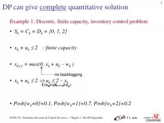
DP can give complete quantitative solution • Example 1: Discrete, finite capacity, inventory control problem • Sk = Ck = Dk = {0, 1, 2} • xk + uk 2 : finite capacity • xk+1 = max(0, xk + uk – wk ) • xk + uk 2 uk 2 – xk • Prob{wk=0}=0.1, Prob{wk=1}=0.7, Prob{wk=2}=0.2 no backlogging U(xk)={0,…,2-xk) ECES 741: Stochastic Decision & Control Processes – Chapter 1: The DP Algorithm
DP can give complete quantitative solution • Example 1 continued: Inventory control problem • N = 3 • gn(xn) = 0 • gk(xk, uk, wk) = uk + 1∙max(0, xk + uk – wk) + 3∙max(0, wk + xk – uk) holding lost demand order ECES 741: Stochastic Decision & Control Processes – Chapter 1: The DP Algorithm
DP can give closed-form solution • Example 2: A gambling model • A gambler is going to bet in N successive plays. The gambler can bet any (nonnegative) amount up to his present fortune. What betting strategy maximizes his final fortune? • P(lose) = p, P(win) = 1 – p = q : Bernoulli • Solution: For convenience, and with no loss in generality, we look to maximize the log of the final fortune. The model is as follows. • Utility of fortune 1 / wealth • U(x) = log(x) : also Bernoulli! ECES 741: Stochastic Decision & Control Processes – Chapter 1: The DP Algorithm
DP can give closed-form solution • Example 2 continued: Variable definitions • xk = fortune at beginning of kth play (after outcome of (k – 1)th play, before kth) • uk = bet for kth play as a percentage of xk • 1 : win w.p. p • -1 : lose w.p. q = 1 – p • gk(xk, uk, wk) = 0, 0 k N – 1 • gN(xN) = -log(xN) • xk+1 = xk + wk uk xk • wk = to maximize ECES 741: Stochastic Decision & Control Processes – Chapter 1: The DP Algorithm
DP can give closed-form solution Example 2 continued: DP algorithm for the problem ECES 741: Stochastic Decision & Control Processes – Chapter 1: The DP Algorithm
DP can give closed-form solution Example 2 continued: Solving the DP at k=N-1 Thus, ECES 741: Stochastic Decision & Control Processes – Chapter 1: The DP Algorithm
DP can give closed-form solution Example 2 continued: Solving the DP at k=N-1 Thus, : consider uN-1 = 1 separately if p = 1 (q = 0) u*N-1 = 1 : bet it all! u*N-1 = p – q if 0 ≤ p < ½, then u*N-1 = 0 (p < q q log(1 – uN-1) dominates) p log(1 + uN-1)+ q log(1 – uN-1)< q log(1 – u2N-1) ≤ 0 ECES 741: Stochastic Decision & Control Processes – Chapter 1: The DP Algorithm
DP can give closed-form solution Example 2 continued: Closed-form solution for k=N-1 Hence, C 0 ECES 741: Stochastic Decision & Control Processes – Chapter 1: The DP Algorithm
DP can give closed-form solution Example 2 continued: Closed-form solution for k=N-1 Hence, can view these as constant functions (controls = percentage) or as feedback policies (total bet ) ECES 741: Stochastic Decision & Control Processes – Chapter 1: The DP Algorithm
DP can give closed-form solution Example 2 continued: Solving the DP at k=N-2 Proceeding one stage (play) back: But except for constant C, this is the same equation as for k = N – 1 solution the same, plus consant C ECES 741: Stochastic Decision & Control Processes – Chapter 1: The DP Algorithm
DP can give closed-form solution Example 2 continued: General closed-from DP solution ECES 741: Stochastic Decision & Control Processes – Chapter 1: The DP Algorithm
DP can be used to obtain qualitative properties (structure) of optimal solutions • Example 3: A stock option model • xk : price of a given stock at beginning of kth day • xk+1 = xk + wk = • {wk} i.i.d., wk ~ F( ) • Random Walk ECES 741: Stochastic Decision & Control Processes – Chapter 1: The DP Algorithm
DP can be used to obtain qualitative properties (structure) of optimal solutions • Example 3 continued: A stock option model • Actions: Have an option to buy one share of the stock at fixed price c; N days to exercise option. If you buy when stock’s price is s: • s – c =profit (can be negative) • What strategy maximizes profit? • Terminating Process (Bertsekas, Prob. 8, Ch. 1) ECES 741: Stochastic Decision & Control Processes – Chapter 1: The DP Algorithm
DP can be used to obtain qualitative properties (structure) of optimal solutions Example 3 continued: Solution ECES 741: Stochastic Decision & Control Processes – Chapter 1: The DP Algorithm
DP can be used to obtain qualitative properties (structure) of optimal solutions • Example 3 continued: Solution • However, process terminates (see prob. 8, ch. 1) when uk=B • introduce fictitious termination state T s.t. mixed symbolic and numeric states discrete event system ECES 741: Stochastic Decision & Control Processes – Chapter 1: The DP Algorithm
DP can be used to obtain qualitative properties (structure) of optimal solutions Example 3 continued: Solution Cost structure changed to: There is no simple analytical solution for Jk(xk) or u*k=*(xk), but we can obtain some qualitative properties (structure) of solutions. ECES 741: Stochastic Decision & Control Processes – Chapter 1: The DP Algorithm
DP can be used to obtain qualitative properties (structure) of optimal solutions Example 3 continued: DP algorithm for the problem uN – 1 = B uN – 1 = DB uk = DB uk = B expected “profit-to-go” ECES 741: Stochastic Decision & Control Processes – Chapter 1: The DP Algorithm
DP can be used to obtain qualitative properties (structure) of optimal solutions • Example 3 continued: Lemma (Ross) • (i) Jk+1(xk) – xk + c is decreasing in xk • after a certain value of stock price profit-to-go is negative buy none • (ii) Jk(xk) is increasing and continuous in xk (backward induction) constant does not affect property ECES 741: Stochastic Decision & Control Processes – Chapter 1: The DP Algorithm
DP can be used to obtain qualitative properties (structure) of optimal solutions Example 3 continued: Theorem (Ross) There exists numbers s1 ≤ s2 ≤ … ≤ sN-k ≤ … ≤sN such that where, These results can be used to solve the problem numerically, or to gain insight into the process. critical stock price values k periods remaining ECES 741: Stochastic Decision & Control Processes – Chapter 1: The DP Algorithm
DP for deterministic problems Example 3 continued: Remark For a deterministic situation, optimizing over policies (feedback) results in no advantage over optimizing over actions (sequences of controls/decisions) Hence, the optimization problem can be solved using linear/nonlinear programming. Furthermore, for a finite state and action deterministic problem, we can equivalently formulate the problem as a shortest path problem for an acyclic graph. ECES 741: Stochastic Decision & Control Processes – Chapter 1: The DP Algorithm
. . . cij 1 c01 0 . . . c02 2 0 start End (Artificial) . . . c03 0 3 k=0 k=1 k=2 k=N-1 k=N DP for deterministic problems • Example 3 continued: Forward search • There are efficient ways to find shortest path, e.g. Branch and Bound algorithms. However, DP has some advantages: • always leads to global optimum • can handle difficult constraint sets ECES 741: Stochastic Decision & Control Processes – Chapter 1: The DP Algorithm
DP can handle difficult constraint sets Example 4: Integer-valued variables Remark: reachable set from x0 = 1 is Z2 : no cost at final stage N=2 ECES 741: Stochastic Decision & Control Processes – Chapter 1: The DP Algorithm
DP can handle difficult constraint sets Example 4 continued: Solution k = 2 k = 1 one-stage cost J2 singleton ECES 741: Stochastic Decision & Control Processes – Chapter 1: The DP Algorithm
DP can handle difficult constraint sets Example 4 continued: Solution k = 0 ECES 741: Stochastic Decision & Control Processes – Chapter 1: The DP Algorithm
DP can handle difficult constraint sets Example 4 continued: Optimal Policy k = 0 ECES 741: Stochastic Decision & Control Processes – Chapter 1: The DP Algorithm