How to create Log Plots

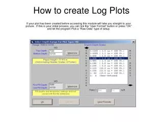
1. How to create Log Plots If your plot has been created before accessing this module will take you straight to your picture. If this is your initial process, you can lick the “User Format” button or press “OK” and let the program Pick a “Raw Data” type of setup.

2. Your Initial Log Plot using program defaults will look something like this. To access “Curve Setup” click this button Or click any curve in the scale area to active setup with the selected curve’s properties showing.

3. Your setup menu will appear in the center of the screen. You will be able to see the underlying Scales and plotted curves before accessing the setup.

4. These are the defined areas of Setup. 1) Toolbar 2) Options when adding new curves 3) Selection Tree for new curves 4) Scales area includes four active areas by clicking your mouse 6) Curve Properties Tab 7) Depth Tracks Tab Is selectable when any curve is displayed 8) Shading Tab with separate left and/or right shading options 5) Curve selection buttons

5. Active Scales & Miscellaneous In this picture the “Max Tracks” was increase to 4 for more visible tracks. If nothing is in the tracks when you press OK it will be hidden in the plot Plot width resizes your picture then same as in the Grid setup after you press OK The Expand button was pressed to show all “Available Curves” in the selection tree • Each curve in the scales has 4 distinct areas to allow for changes or focus • Curve Section: shows curve properties • Line Type: click to toggle to desired type • Line Color: a color Box will appear • Line thickness: click to toggle thickness Drag new curves to this area below the last shown curve line for all tracks

6. 1) The Toolbar OK: saves changes you have made as does the close icon at the right of on the title bar Cancel: Ignores all changes you have made while this form was visible Add: is inactive until a curve is selected in the tree. Curves will be added to the last Plot Track for the Curve properties shown. Also you can click the curve and when it has a box around it then drag it to the desired track. New curves are currently being added to this track Delete: Click the curve int the Scales Area then click the Delete button. You may also drag the curve from the Scales area And drop it on the Delete to remove it. Copy: This will make a copy of the selected curve and all it’s properties asking you which track to place it in. Undo: This undoes your last change. There number of changes made to this shown is shown in brackets as they are made.

7. 2) Options When Adding New Curves The options in this section only apply when adding new curves to your Scales. Low: for Low porosity logs Phi is set to 30 - 10 and Resistivity is set to .2-2000 and RhoB is set to 2 - 3 Med:. for Medium porosity logs Phi is set to 45 - -15 and Resistivity is set to .2-200 and RhoB is set to 1.95 - 2.95 High: for High porosity logs Phi is set to 60 - 0 and Resistivity is set to .2-20 and RhoB is set to 1.65 - 2.65 Use Scales already in Plot: sees if a curve of this type already exists and copies the properties from it. Drag new curves to this area for Track 4 Drag new curves to this area for the next open track which in this case ins no. 5

8. Toolbar - Options Reverse Scales: swaps left & right scales for active curve. Reverse All In Tracks: swaps left & right scales for all curves in active track. Equalize Scales: takes the left and right scales of the active curves and changes all similar type curves in the same track to these values. Match Grid to Curve: The last two options only apply to Logarithmic scales. This option forces the “Grid Lines” cycles to match the active curve. Match Curve to Grid: This option forces the active curve left & right to match the properties set for the “Grid Lines” cycles. These buttons only show with Logarithmic curves and correspond to the Options buttons

9. 3) Selection Tree The expanded mode shows all available curves in your file by groupings. You may add any of these cures. Collapsed mode shows only major catagories. These cannot be added to a track. • Click the curve, then press the Add button on the tool bar • Or Click and drag the box to the desired area. NOTE: the curve will not drag without the box around it.. The sort button does an alpha sort to the Major braches only.

10. 4) The Scale Display area Click any curve name for it’s properties B A Point A: You may also click in the bottom open area of any track and drop it to the left of where you want to place it Point B: is desired position Point C: is resulting picture.. 5) Use these Curve Section buttons to toggle through the settings. C

11. 6) Curve Properties Tab These areas do the same process.

12. 7) Depth Tracks Tab This tab may be accessed while editing any curve. These are the same properties you will see in the Grid Setup form. Use this tab to create another depth track or to show additional depth references. You may also change the position numerically or dragging it to the left of where you want to place It.

13. 8) Left / Right Shading Tabs One of the newer features is the abiltiy to fill to the left or the right. In this case GR is the active curve. There are both a frame for different Left & Right properties. In this case, we are filling left to a value of 10, although you could select the track border or the CALI in this track. Title: is optional to let you describe what is being filled. Ex: Gas, Oil, Water etc. • Color Style • Solid using the Colo box. • Custom Shading using the gamma ray for an appearance of lamination. • Patterns allows you to select any lithology pattern on your list Apply filters: alows you to start and stop the fill in areas where you have washout , porsosity gets to low etc. This is similar to a pay filter in action.

14. GR Fill Example • Right Shading • From the Curve to the Track Border. • Fill title is “Clean Sands” • Color style is Custom using GR a axis • There are no filters applied. • Left Shading • From the Curve to a value of 10 • No Title is selected. • Color style is the Shale pattern • There are no filters applied.

15. 9) Lithology Tab When lithology is the active curve, the Left/Right Shading tab is hidein and the Lithology tab is displayed. The choices here are self explanatory by clicking the items. Active Curve

16. Extended and Split Tracks Example PEF: is in Track 2 only in the Left Half Sw: is in Track 2 only in The Right Half PHiE: is in Track 2 over the Full Track TNPH: is in Tracks 2-3 (extended over Tracks 2 & 3). Normal Tracks: 1 2 3 4 5 6 7 8 Extended Tracks: 1-2 2-3 3-4 4-5 5-6 6-7 7-8 Depth Tracks: 0 (capable of holding curves) 9 (optional depth references)