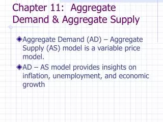
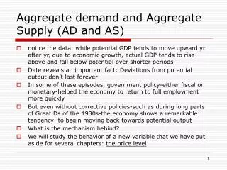
Aggregate demand and Aggregate Supply (AD and AS)

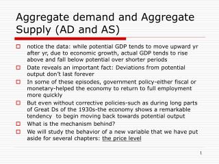
1. Aggregate demand and Aggregate Supply (AD and AS) • notice the data: while potential GDP tends to move upward yr after yr, due to economic growth, actual GDP tends to rise above and fall below potential over shorter periods • Date reveals an important fact: Deviations from potential output don’t last forever • In some of these episodes, government policy-either fiscal or monetary-helped the economy to return to full employment more quickly • But even without corrective policies-such as during long parts of Great Ds of the 1930s-the economy shows a remarkable tendency to begin moving back towards potential output • What is the mechanism behind? • We will study the behavior of a new variable that we have put aside for several chapters: the price level

2. 9,000 The orange line shows full-employment or potentialoutput. 8,000 7,000 Actual and Potential Real GDP (Billions of 1996 Dollars) 6,000 The green line showsactualoutput. During recessions, output declines. 5,000 4,000 During expansions, output rises—sometimes rapidly. 3,000 2,000 1960 1965 1970 1975 1980 1985 1990 1995 2000 2003 Figure 1a: Potential and Actual Real GDP, 1960-2001

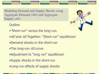
3. Aggregate Demand Curve Price Real Level GDP Aggregate Supply Curve Figure 1: The Two-Way Relationship Between Output and the Price Level

4. AD and AS • There exist a two-way relationship between price level and output (see diagram 1) • Changes in price level cause changes in real GDP – illustrated by Aggregate Demand curve • Changes in real GDP cause changes in price level – illustrated by Aggregate Supply curve

5. The Aggregate Demand Curve • First step in understanding how price level affects economy is an important fact • When price level rises, money demand curve shifts rightward (because purchases become more expensive) • Shift in money demand, and its impact on the economy, is illustrated in Figure 2 • Imagine a rather substantial rise in price level—from 100 to 140 • Compared with our initial position, this new equilibrium has the following characteristics • Money demand curve has shifted rightward • Interest rate is higher • Aggregate expenditure line has shifted downward • Equilibrium GDP is lower • All of these changes are caused by a rise in price level • A rise in price level causes a decrease in equilibrium GDP

6. Interest Rate As the price level rises, money demand increases and interest rate rises. 9% 6% Money ($ Billions) Figure 2a: Deriving the Aggregate Demand Curve (a) Ms H E 500

7. On the AD curve, a higher price level is associated with a lower real GDP. The rise in the interest rate causes real GDP to fall. Figure 2b/c: Deriving the Aggregate Demand Curve (c) (b) Price Level AEr = 6% H AEr= 9% 140 E Aggregate Expenditure ($ Trillions) E 100 H AD Real GDP ($ Trillions) Real GDP ($ Trillions) 6 10 6 10

8. Deriving the Aggregate Demand Curve • Panel (c) of Figure 2 shows a new curve • Shows negative relationship between price level and equilibrium GDP • Call aggregate demand curve • Tells us equilibrium real GDP at any price level

9. Understanding the AD Curve • AD curve is unlike any other curve you’ve encountered in this text • In all other cases, our curves have represented simple behavioral relationships • But AD curve represents more than just a behavioral relationship between two variables • Each point on curve represents a short-run equilibrium in economy • A better name for AD curve would be “equilibrium output at each price level” curve—not a very catchy name • AD curve gets its name because it resembles demand curve for an individual product • AD curve is not a demand curve at all, in spite of its name

10. Movements Along the AD Curve • As you will see later in this chapter, a variety of events can cause price level to change, and move us along AD curve • Suppose price level rises, and we move from point E to point H along this curve • Following sequence of events occurs • Opposite sequence of events will occur if price level falls, moving us rightward along AD curve

11. Shifts of the AD Curve • When we move along AD curve in Figure 2, we assume that price level changes • But that other influences on equilibrium GDP are constant • Keep following rule in mind • When a change in price level causes equilibrium GDP to change, we move along AD curve • Whenever anything other than price level causes equilibrium GDP to change, AD curve itself shifts • Equilibrium GDP will change whenever there is a change in any of the following • Government purchases • Autonomous consumption spending • Investment spending • Net exports • Taxes • Money supply

12. An Increase in Government Purchases • Spending shocks initially affect economy by shifting aggregate expenditure line • In Figure 3, we assume economy begins at a price level of 100 • Let’s increase government purchases by $2 trillion and ask what happens if price level remains at 100 • An increase in government purchases shifts entire AD curve rightward • AD curve shifts rightward when government purchases, investment spending, autonomous consumption spending, or net exports increase, or when taxes decrease • Analysis also applies in the other direction • AD curve shifts leftward when government purchases, investment spending, autonomous consumption spending, or net exports decrease, or when taxes increase

13. Since real GDP is higher at the given price level, the AD curve shifts rightward. At any given price level, an increase in government purchases shifts the AE line upward, raising real GDP. Figure 3: A Spending Shock Shifts the AD Curve (a) (b) Price Level AE2 AE1 H Real Aggregate Expenditure ($ Trillions) 100 H E E AD1 AD2 Real GDP ($ Trillions) Real GDP ($ Trillions) 10 13.5 10 13.5

14. Changes in the Money Supply • Changes in money supply will also shift aggregate demand curve • Imagine that Fed conducts open market operations to increase money supply • AD curve shifts rightward • A decrease in money supply would have the opposite effect

15. Shifts vs. Movements Along the AD Curve: A Summary • Figure 4 summarizes how some events in economy cause a movement along AD curve, and other events shift AD curve • Panels (b) and (c) of Figure 4 tell us how a variety of events affect AD curve, but not how they affect real GDP • Where will price level end up? • First step in answering that question is to understand the other side of the relationship between GDP and price level

16. Price level ↑ moves us leftward along the AD curve Price level ↓ moves us rightward along the AD curve Figure 4a: Effects of Key Changes on the Aggregate Demand Curve (a) Price Level P3 P1 P2 AD Real GDP Q3 Q1 Q2

17. Entire AD curve shifts rightward if: • a, IP, G, orNXincreases • Net taxes decrease • The money supply increases Figure 4b: Effects of Key Changes on the Aggregate Demand Curve (b) Price Level AD2 AD1 Real GDP

18. Entire AD curve shifts leftward if: • a, IP, G, orNXdecreases • Net taxes increase • The money supply decreases Figure 4c: Effects of Key Changes on the Aggregate Demand Curve (c) Price Level decreases AD1 AD2 Real GDP

19. Costs and Prices • Price level in economy results from pricing behavior of millions of individual business firms • In any given year, some of these firms will raise their prices, and some will lower them • But often, all firms in the economy are affected by the same macroeconomic event • Causing prices to rise or fall throughout the economy – what interest us in macroeconomics • To understand how macroeconomic events affect the price level, we begin with a very simple assumption • A firm sets price of its products as a markup over cost per unit

20. Costs and Prices • Percentage markup in any particular industry will depend on degree of competition there • In macroeconomics, we are not concerned with how the markup differs in different industries • But rather with average percentage markup in economy • Determined by competitive conditions • Competitive structure changes very slowly, so average percentage markup should be somewhat stable from year-to-year • But a stable markup does not necessarily mean a stable price level, because unit costs can change • In short-run, price level rises when there is an economy-wide increase in unit costs • Price level falls when there is an economy-wide decrease in unit costs

21. GDP, Costs, and the Price Level • Primary concern here: impact of real GDP on unit costs and, therefore, on the price level • Why should a change in output affect unit costs and price level? • As total output increases • Greater amounts of inputs may be needed to produce a unit of output • Price of non-labor inputs rise • Nominal wage rate rises • A decrease in output affects unit costs through the same three forces, but with opposite result

22. The Short Run • All three of our reasons are important in explaining why a change in output affects price level • However, they operate within different time frames • But our third explanation—changes in nominal wage rate—is a different story • For a year or more after a change in output, changes in average nominal wage are less important than other forces that change unit costs • Some of the more important reasons why wages in many industries respond so slowly to changes in output • Many firms have union contracts that specify wages for up to three years • Wages in many large corporations are set by slow-moving bureaucracies • Wage changes in either direction can be costly to firms • Firms may benefit from developing reputations for paying stable wages

23. The Short Run • Nominal wage rate is fixed in short-run • We assume that changes in output have no effect on nominal wage rate in short-run • Since we assume a constant nominal wage in short-run, a change in output will affect unit costs through the other two factors • In short-run, a rise (fall) in real GDP, by causing unit costs to increase (decrease), will also cause a rise (decrease) in price level

24. Deriving the Aggregate Supply Curve • Figure 5 summarizes discussion about effect of output on price level in short-run • Each time we change level of output, there will be a new price level in short-run • Giving us another point on the figure • If we connect all of these points, we obtain economy’s aggregate supply curve • Tells us price level consistent with firms’ unit costs and their percentage markup at any level of output over short-run • A more accurate name for AS curve would be “short-run-price-level-at-each-output-level” curve

25. Starting at point A, an increase in output raises unit costs. Firms raise prices, and the overall price level rises. Starting at point A, a decrease in output lowers unit costs. Firms cut prices, and the overall price levelfalls. Figure 5: The Aggregate Supply Curve Price Level AS 130 B 100 A 80 C Real GDP ($ Trillions) 6 10 13.5

26. Movements Along the AS Curve • When a change in output causes price level to change, we move along economy’s AS curve • What happens in economy as we make such a move? • As we move upward along AS curve, we can represent what happens as follows

27. Shifts of the AS Curve • Figure 5 assumed that a number of important variables remained unchanged • But in real world, unit costs sometimes change for reasons other than a change in output • In general, we distinguish between a movement along AS curve, and a shift of curve itself, as follows • When a change in real GDP causes the price level to change, we move along AS curve • When anything other than a change in real GDP causes price level to change, AS curve itself shifts • What can cause unit costs to change at any given level of output? • Changes in world oil prices • Changes in the weather • Technological change • Nominal wage, etc.

28. When unit costs rise at any given real GDP, the AS curve shifts upward–e.g., an increase in world oil prices or bad weather for farm production. Figure 6: Shifts of the Aggregate Supply Curve AS2 Price Level AS1 L 140 100 A Real GDP ($ Trillions) 10

29. Real GDP ↑ moves us rightward along the AS curve Real GDP ↓ moves us leftward along the AS curve Figure 7a: Effects of Key Changes on the Aggregate Supply Curve (a) Price Level AS P3 P1 P2 Real GDP Q2 Q1 Q3

30. Entire AS curve shifts upward if unit costs ↑ for any reason besides an increase in real GDP Figure 7b: Effects of Key Changes on the Aggregate Supply Curve (b) AS2 Price Level AS1 Real GDP

31. Entire AS curve shifts downward if unit costs ↓ for any reason besides an decrease in real GDP Figure 7c: Effects of Key Changes on the Aggregate Supply Curve (c) Price Level AS1 AS2 Real GDP

32. AD and AS Together: Short-Run Equilibrium • Where will the economy settle in short-run? • Where is our short-run macroeconomic equilibrium? • We know that in equilibrium, economy must be at some point on AD curve • Short-run equilibrium requires economy be operating on its AS curve • Only when economy is at point E—on both curves—will we have reached a sustainable level of real GDP and the price level

33. Figure 8: Short-Run Macroeconomic Equilibrium AS Price Level B 140 E 100 F AD Real GDP ($ Trillions) 6 10 14

34. What Happens When Things Change? • Now that we know how short-run equilibrium is determined, and armed with our knowledge of AD and AS curves, we are ready to put model through its paces • Our short-run equilibrium will change when either AD curve, AS curve, or both, shift • An event that causes AD curve to shift is called a demand shock • An event that causes AS curve to shift is called a supply shock • In earlier chapters, we’ve used phrase spending shock • A change in spending by one or more sectors that ultimately affects entire economy • Demand shocks and supply shocks are just two different categories of spending shocks

35. An Increase in Government Purchases • Shifts AD curve rightward • Can see how it affects economy in short-run: increases output and rises interest rate in the money market • Process described is not entirely realistic • Assumes that when government purchases rise, first output increases, and then price level rises • In reality, output and price level tend to rise together

36. Figure 9: The Effect of a Demand Shock AS Price Level 130 H 115 J 100 E AD2 AD1 Real GDP($ Trillions) 10 13.5 12.5

37. An Increase in Government Purchases • Can summarize impact of price-level changes • When government purchases increase, horizontal shift of AD curve measures how much real GDP would increase if price level remained constant • But because price level rises, real GDP rises by less than horizontal shift in AD curve

38. An Decrease in Government Purchases

39. An Increase in the Money Supply • Although monetary policy stimulates economy through a different channel than fiscal policy • Once we arrive at AD and AS diagram, two look very much alike • Can represent situation as follows

40. Other Demand Shocks • A positive demand shock—shifts AD curve rightward • Increases both real GDP and price level in short-run • A negative demand shock—shifts AD curve leftward • Decreases both real GDP and price level in short-run

41. An Example: The Great Depression • U.S. economy collapsed far more seriously during 1929 through 1933—the onset of the Great Depression—than it did at any other time • What do we know about demand shocks that caused Great Depression? • Fall of 1929, bubble of optimism burst • Stock market crashed, and investment and consumption spending plummeted • Demand for products exported by United States fell • Fed reacted by cutting money supply sharply • Each of these events contributed to a leftward shift of AD curve • Causing both output and price level to fall

42. Demand Shocks: Adjusting to the Long-Run • In Figure 9, point H shows new equilibrium after a positive demand shock in short-run—a year or so after the shock • But point H is not necessarily where economy will end up in long-run • In short-run, we treat wage rate as given • But in long-run, wage rate can change • When output is above full employment, wage rate will rise, shifting AS curve upward • When output is below full employment, wage rate will fall, shifting AS curve downward

43. Demand Shocks: Adjusting to the Long Run • Increase in government purchases has no effect on equilibrium GDP in long-run • Economy returns to full employment, which is just where it started • This is why long-run adjustment process is often called economy’s self-correcting mechanism • If a demand shock pulls economy away from full employment • Change in wage rate and price level will eventually cause economy to correct itself and return to full-employment output

44. Figure 10: The Long-Run Adjustment Process Price Level AS2 AS1 P4 K J P3 P2 H P1 E AD2 AD1 YFE Y3 Y2 Real GDP

45. Demand Shocks: Adjusting to the Long Run • For a positive demand shock that shifts AD curve rightward, self-correcting mechanism works like this

46. Figure 11: Long-Run Adjustment After A Negative Demand Shock Price Level AS1 AS2 P1 E P2 N P3 M AD1 AD2 Real GDP Y2 YFE