Download
1 / 37
370 likes | 473 Views
Review of Aggregate Supply & Aggregate Demand. Overview of AS-AD. Simple model of Aggregate Supply and Aggregate Demand Same idea as supply and demand AD slopes down: As price rises AD falls summarizes the whole of the IS-LM-BP model AS slopes up: As price rises AS increases

E N D
Overview of AS-AD • Simple model of Aggregate Supply and Aggregate Demand • Same idea as supply and demand • AD slopes down: • As price rises AD falls • summarizes the whole of the IS-LM-BP model • AS slopes up: • As price rises AS increases • Expectations are important
AS P AD Y
Example: Fiscal Policy P AS • If G increases then AD shifts to right • At any P, AD will be higher because G is higher • P and Y rise • Why P rise? • Need to pay higher w to get higher output B A AD1 ADo Y
Aggregate Supply • Q: What underlies the Aggregate Supply Curve? • A: Labour market • Why? – to increase production • hire more people • Pay higher wages • More of other inputs also • Focus on labour market
Labour Market W • Firms have a demand for labour • Decreases as wage rises • Increases as Price of output rises • Curve shifts to the right • At any wage firm will want more workers D1 Do L
W • Workers supply labour • Form expectation about cost of living • Price expectation (Pe) • Higher wage will induce more work(ers) • Increased (Pe) • Curve shifts up • Higher wage for any level of work L
Labour market Equilibrium W S(Pe) • Put two curves together • Lab Mkt eqm • Firms and workers plans agree • Wage and employment • Also agree on price • P=Pe • Rational expectations • Implies agree on real wages D(P) L
Derive the Aggregate Supply Curve • We can use the labour market to derive the AS curve in short run and in the long run • First the short run: • Assume that expectations do not change • Pe = P • SL will not move
Suppose start at A which represents lab mkt eqm • P level rises • DL increases • New eqm at B • Employment increases • Wage increases • Goods market • Output increases • Upward sloping supply curve • Note that AS depends on expectations
SL(Pe) W P AS(Pe) B B A DL(P1) A DL(P0) L Y
Note that all this implies something weird about workers • The work more, for less! • W has increased, but P has increased by more • Real wages have declined • See diagram • Supply of labour was conditional on prices being at a certain level • Pe = P • But this no longer true
With P>Pe we have • Demand w increase to restore living standards • they adjust expectations upwards • Supply curve shifts up • Shifts up so that increase in W is same as increase in P • New equilibrium is a point C • Real wage same at C as at A • Employment same at C as at A
SL(Pe) AS(Pe) C SL(Pe) W P AS(Pe) B C B A DL(P1) A DL(P0) L Y
As expectations change there is a new AS curve • Eqm at C has same output as A • Reflects the fact that employment is the same • Net effect is that output and employment remain the same • P and W go up by the same amount
Summary of AS • We have a distinction between short run and long run • The Short run is for fixed expectations • AS(Pe) • SRAS • Quite flat: Explains why ISLM works as approx • LR is how long it takes for real wages to adjust • Expectations adjust • Workers to act on exp • ISLM wont work in LR • In LR Y is unaffected by P
LRAS P AS(Pe) Y* Y
What determines Y*? • Natural rate • Incentives • Technology • “growth” • Not anything that just affects price
Policy in AS-AD Model • Suppose there is an increase in G • AD shifts right • For all P, there is higher AD, because govt component has risen • Could derive this from IS-LM • Same for MP • For fixed expectations i.e. SR • Move along AS • New (temp) eqm at B • Y increases • P increases (but not by much)
P rising implies real wage falling • P>Pe • Pe will adjust upwards • W increase • SRAS shifts up • Keep going until output returns to “natural level” • How long does transition take? • Theory: depends. Instantaneous? • Empirics: about 2 years – see diagram
LRAS P C AS(Pe) B A AD1 AD0 Y* Y
Be clear on the reasons why there is no long run effect • In order to get more output need to pay more people higher wages • Higher wages imply firms need to charge higher prices • Higher prices negate the higher wages as far as workers are concerned • We go back to original values of real variables • Only affect nominal variables • Policy is ineffective!
We can only get an increase in Y in long run i.e. increase in Y* • If induce people to work more • Need increase in real wage • Technology • Efficiency • Lower taxes? • Reganomics • Supply side economics • Voodoo economics
Reagan Style Tax Cut • Cut personal taxes • Idea is that this will improve incentives • People will work more • Shift the LRAS to the right • Increase Y* and reduce P • Note that SRAS shifts also as expectations adjust to the new lower level • But cutting taxes will shift the AD curve to right • SR boom • LR return to Y* with higher P • Which happened? • Both • Demand effect larger
P LRAS AS(Pe) AS(Pe) A B AD0 Y* Y
Dealing With Shocks • The AS-AD diagram shows how an economy will automatically adjust to a shock • Re-adjust to be in terms of inflation • Start from LR eqm • Y=Y* • pe=p • Suppose there is a fall in AD • Eqm moves from A to B • Y<Y* • This can only be a temporary eqm
At B, p<pe • Real wages are higher than expected • Prices fall, but by more than nominal wages • See labour market diagram • Workers are expensive • Explains the decline in output • Over time workers will • Reduce price expectations • Reduce wage demands • SRAS shifts down • Process continues until LR eqm is restored at C • Real wage returns to original level • Y=Y* • pe=p but at new lower level
LRAS p SRAS(pe) A B C AD0 AD1 Y* Y
So the economy will automatically work itself out of recession • Mechanism depends on wage adjustment • Mirror image of previous discussions • Workers respond to lower prices by demanding lower wages • Reasonable? • Yes real wages return to normal • No long term decline in real wages • Realistic? • No! see data • Nominal wages are rigid • Have to wait for productivity • Have lower wage increases than otherwise
All this takes time • 3+ years • Alternative is for Government to expand AD • Shift AD back • Return to long run equilibrium A • Rationale for stabilization policy • After WTC, cut interest rates • Enough? Or too much? • Debate over which is best • Policy: “long and variable lags” • Automatic: “long run we are all dead” • Calls for “flexibility” after EMU
Disinflation • We can use the model to analyse the issue of deflation • i.e. how do we lower inflation without causing (much) unemployment (lower output) • This is the flip-side of what we just looked at • What happens when we try to reduce unemployment • We already know part of the answer • LR there is no trade-off • No LR increase in unemployment (or loss of output) • SR there is a trade off • Reducing inflation will mean higher U (lower Y) • Expectations play a role
LRAS p SRAS(pe) A B C AD0 AD1 Y* Y
Suppose we are at A • Unemployment equals its natural rate (6%) • Inflation is 12% • Too high want to reduce it • Reduce AD (increase interest rates) • Unemployment rises: 8% > 6% • Move down the SRAS to B • Actual inflation falls • B cannot be LR eqm (why?) • Actual Inflation (9%) is lower than expected (12%) • Real wages higher than expected • Expectations adjust down – • New SRAS
New SR eqm at C • Still not a LR equilibrium • Inflation will keep falling for as long as U is kept above the natural rate • When the gov. is satisfied with the level of inflation, • allow unemployment to return to the natural rate • Inflation stable
Disinflation achieved at a cost • Y<Y* for several years • Sacrifice ratio • The increase in unemployment (above the natural rate) needed to reduce inflation by one percentage point in one year. • My example: 0.66 • Example Volker disinflation • Inflation fell by 6.7% over 4 years (1982-85) • Unemployment was 9.5%, 9,5%, 7.4% and 7.1% • Natural rate was 6% • Sacrifice ratio 1.4
Painless Disinflation • Previous example assumed expectations adjust gradually • In reality expectations could adjust a lot quicker • Think of extreme case • Expectations adjust fully and immediately • Full immediate fall in inflation without any increase in unemployment • Sacrifice ration of zero
What is required for this? • Policy must be announced • Policy must be credible • Willing to cause pain • Intermediate case is more realistic • More credible policy maker faces a lower sacrifice ratio