Download
1 / 26
260 likes | 411 Views
This text explores the dynamic control of energy systems, focusing on O.D.E. solution techniques such as direct integration, exponential solutions, and Laplace transforms, which help determine the time response of systems described by differential equations. It covers both the free and forced responses of a first-order model, detailing the conversion to the time domain, system time constants, and the meanings of stability and instability. Furthermore, it discusses various input models like step, pulse, impulse, and ramp inputs, along with the use of transfer functions to analyze forced responses in Laplace domain.

E N D
System Response Characteristics ISAT 412 -Dynamic Control of Energy Systems (Fall 2005)
Review • We have overed several O.D.E. solution techniques • Direct integration • Exponential solutions (classical) • Laplace transforms • Such techniques allow us to find the time response of systems described by differential equations
Generic 1st order model • Solution in Laplace domain • Solution comprised of • Free Response (homogeneous solution) • Forced Response (non-homogeneous solution)
Free response of 1st order model • Free response means: • Converting back to the time domain:
Time constant • Define the system time constant as • Rewriting the free response or
Free response behavior Unstable Stable Unstable
Meaning of the time constant • When t = t • When t = 2t, t = 3t, and t = 2t,
Transfer Functions and Common Forcing Functions ISAT 412 -Dynamic Control of Energy Systems (Fall 2005)
Forced response of 1st order system • The forced response corresponds to the case where x(0) = 0 • In the Laplace domain, the forced response of a 1st order system is
Transfer functions • Solve for the ratio X(s)/F(s) • T(s) is the transfer function • Can be used as a multiplier in the Laplace domain to obtain the forced response to any input
Using the transfer function • Now that we know the transfer function for a 1st order system, we can obtain the forced response to any input if we can express that input in the Laplace domain
Step input • Used to model an abrupt change in input from one constant level to another constant level • Example: turning on a light switch
Heaviside (unit) step function • Used to model step inputs
Time shifted unit step function • For a unit step shifted in time, • Using the shifting property of the Laplace transform (property 6)
Step input model • For a step of magnitude b at time D
Pulse input model • Use two step functions
Pulse input model • For a pulse input of magnitude M, starting at time A and ending at time B
Impulse input • Examples: explosion, camera flash, hammer blow
Impulse input model • Unit impulse function • For an impulse input of magnitude M at time A
Ramp input model • For a ramp input beginning at time A with a slope of m
Other input functions • Sinusoidal inputs • Combinations of step, pulse, impulse, and ramp functions
Square wave input model • Addition of an infinite number of step functions with amplitudes A and -A