Abstract

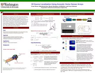
1. Acoustic vector sensor (AVS) Pressure sensor Particle velocity sensor 3D Source Localization Using Acoustic Vector Sensor Arrays Evan Nixon, Satyabrata Sen, Murat Akcakaya, Ed Richter, and Arye Nehorai Department of Electrical and Systems Engineering Azimuth and Elevation Estimation Abstract Experimental Setup and GUI Single AVS and source model Data flow in our experimental setup In this project, we use an array of two acoustic vector sensors (AVSs) for 3D localization of a single sound source. For each AVS we first use Capon beamforming, a spatial filtering process, to determine the 3D source direction. Then, we apply a triangulation method to combine the directions, estimated by the array of AVSs, to estimate the location of the source. An AVS is composed of one pressure sensor and three orthogonally positioned velocity sensors. Combining these four measurements, a single AVS can uniquely determine the direction of a source in three-dimensional (3D) space. This is a significant advantage compared with a single pressure-sensor, which cannot estimate 3D source direction. Array of AVS Signal conditioner Matlab LabView DAQ direction of particle velocity and are the azimuth and elevation angles, respectively pressure-sensor-measurement noise particle-velocity-measurement noise Overview • Goal • Estimate the three dimensional position of an sound source using measurements of pressure and particle acoustic fields. • Approach • Statistical analysis of pressure and particle velocity measurements taken by two acoustic vector sensors to triangulate a sound source in three dimensions • Applications • Navigation, defense, leak localization • Background Multiple AVS and single source model Figure: LabView and Matlab integration Figure: the LabView GUI Steering vector Experimental Output After each buffer of data is parsed by LabView and Matlab, Two figures are output to show the estimated position of the source: Scenario: Source position (x,y,z) = (2,12,7)Sensor positions (x,y,z) = (-10,0,0) and (10,0,0)Note: Units are normalized Capon Beamforming The colored spheres to the left show the power spectrum from different angles of arrival. The direction with a red arrow emerging from it is the direction which received the greatest power during the last buffer. The two planar plots to the right of the spheres show the power distribution across azimuth and elevation angles. Capon Spectra sample-correlation matrix for N samples 3D Position Estimation The plot to the left shows the calculated position of a sound source. Each blue line points from the AVS array on the x-axis to the estimated position of the acoustic source. The position of the sound source is found by projecting the directions of arrival of each sensor onto the x-y and x-z planes. Sensor Positions: Sensor 1 (x,y,z) = (-d/2,0,0) , Sensor 2 (x,y,z) = (d/2,0,0) The formulae on the left project the two directions of arrival onto the xy plane and calculate the distance to the source in the x and y directions. After finding the x and y components of the distance to the source, the z distance is calculated using the formula to the left References • A. Nehorai and E. Paldi, ``Acoustic vector sensor array processing," Proc. 26th Asilomar Conf. Signals, Syst. Comput., pp. 192-198, Pacific Grove, CA, Oct. 1992. • A. Nehorai and E. Paldi, "Acoustic vector-sensor array processing," IEEE Trans. on Signal Processing, Vol. SP-42, pp. 2481-2491, Sept. 1994. • M. Hawkes and A. Nehorai, "Acoustic vector-sensor beamforming and capon direction estimation," IEEE Trans. on Signal Processing, Vol. SP-46, pp. 2291-2304, Sept. 1998. , = Azimuth angles measured from sensor 1 and 2 respectively= Elevation angles of the source measured from sensor 1 Figure:Photograph of a three dimensional sound intensity probe consisting of one pressure sensor and three particle velocity sensors mounted together (Source: Microflown Technologies, B.V.) 1 2 1