Download
1 / 113
1.13k likes | 1.45k Views
On Radio Technology. EE206A (Spring 2003): Lecture #3. Mani Srivastava UCLA - EE Department mbs@ee.ucla.edu. Readings for this Lecture. MANDATORY

E N D
On Radio Technology EE206A (Spring 2003): Lecture #3 Mani SrivastavaUCLA - EE Departmentmbs@ee.ucla.edu
Readings for this Lecture • MANDATORY • Eugene Shih, Seong-Hwan Cho, Nathan Ickes, Rex Min, Amit Sinha, Alice Wang, and Anantha Chandrakasan, “Physical Layer Driven Algorithm and Protocol Design for Energy-Efficient Wireless Sensor Networks,” Proceedings of MOBICOM 2001, Rome, Italy, July 2001.http://www-mtl.mit.edu/research/icsystems/uamps/pubs/eugene_mobicom01.html • S. Cui, A. J. Goldsmith and A. Bahai, “Modulation Optimization under Energy Constraints,” to appear at ICC'03, Alaska, U.S.A, May, 2003.http://systems.stanford.edu/Publications/Shuguang/icc03.pdf • RECOMMENED • Evans, J.G.; Shober, R.A.; Wilkus, S.A.; Wright, G.A. A low-cost radio for an electronic price label system. Bell Labs Technical Journal, vol.1, (no.2), Lucent Technologies, Autumn 1996. p.203-15.http://www.lucent.com/minds/techjournal/autumn_96/pdf/paper14.pdf • Terence Barrett, “History of UltraWideBand (UWB) Radar & Communications: Pioneers and Innovators” http://www.ntia.doc.gov/osmhome/uwbtestplan/barret_history_(piersw-figs).pdf • OTHER • Richley, R.A.; Butcher, L. Wireless communications using near field coupling. US Patent 5,437,057, 1995. Search athttp://www.uspto.gov/patft/index.html • Zimmerman, T.G. Personal area networks: near-field intrabody communication. IBM Systems Journal, vol.35, (no.3-4), IBM, 1996. p.609-17.http://www.research.ibm.com/journal/sj/384/zimmerman.html
SourceDecoder SourceCoder SourceDecoder SourceCoder Digital Radio Link antenna MultipleAccess ChannelCoder PowerAmplifier Source Multiplex Modulator Carrier fc transmitted symbol stream Radio Channel Radio Technologyand Trends received (corrupted)symbol stream MultipleAccess ChannelDecoder Demodulator& Equalizer RFFilter Destination Demultiplex antenna Carrier fc
Things You Did Not Want to Know About Digital Communications!
How is Information Communicated? 0 1 0 1 1 1 0 0 1 0 1 0 Information V, I Electrical waveform Electro-magnetic waveform
Digital Modulation & Demodulation • Modulation: maps sequence of “digital symbols” (groups of n bits) to sequence of “analog symbols” (signal waveforms of length TS) • Demodulation: maps sequence of “corrupted analog symbols” to sequence “digital symbols” - e.g. maximum likelihood decision
Grouping the Information Bits into Symbols • If M ∞ the ‘performance’ goes up, but at a cost of complexity (Shannon limit) b bits/symbol = M possible waveforms 1 bit/symbol 0 1 11 10 01 00 2 bits/symbol
Signal Space Representation • The basic idea is that we can transmit information in parallel over a set of orthogonal waveforms with respect to the symbol interval T. The inverse of this interval is called the symbol rate: Rs = 1/T.
s1(t) Sample at t = T s2(t) Detection of the Symbols • Correlation or matched filter detector (basically equivalent)
Commonly Used Modulation Techniques • Coherent or Synchronous Detection • process received signal with a local carrier of the same frequency and phase • e.g. phase shift keying, frequency shift keying, amplitude shift keying, continuous phase modulation • Noncoherent or Envelope Detection • requires no reference wave • e.g. FSK, differential PSK, CPM, ASK
a2 . s1 a2 . s2 a1 . s1 a1 . s2 Amplitude Scaling • Instead of sending only s1, s2, s3 … sL etc. combine these with a set of possible scaling factors a1, a2, a3 … aK s1(t) Sample at t = T X s2(t) Y
s2 s2 s1 s1 s2 s2 s1 s1 Information Mapping Examples M = 4 M = 2 Send s1, s2, both or none of them. Send either s1 or s2. M = 8 M = 4 Send any of these combinations. Send s1 or s2.
f2 f1 Some Elementary Schemes FSK (Frequency Shift Keying) Baseband PAM (Pulse Amplitude Modulation) s1 Passband PAM (Pulse Amplitude Modulation) f1
g(t) Q (ai, bi) I time T 0 Sinusoidal Waveforms Quadrature (Q) In-phase (I) s2 s1
q(t) time T 0 cos(2.fc.t) ai ai . q(t) ai(t) = ai . g(t) si(t) D/A D/A g(t) bi bi(t) = bi . g(t) bi . q(t) -sin(2.fc.t) LPF LPF time T 0 Transmitter Structure
Frequency Domain T 1/T time frequency Baseband BW (bandwidth) fc Passband BW (bandwidth)
ni cos(2.fc.t) ai(t) si(t) bi(t) LPF LPF -sin(2.fc.t) Modulation and Demodulation Modulation Demodulation 2.cos(2.fc.t) a(t) ri(t) b(t) -2.sin(2.fc.t) In flat fading channel
Q ai + j·bi ri i I Alternative Interpretation
QAM and PSK QAM (Quadrature Amplitude Modulation) 64-QAM 16-QAM 4-QAM PSK (Phase Shift Keying) 8-PSK 16-PSK 4-PSK
Example • QAM: Each symbol is represented by a tuple of amplitude and phase • FSK: Each symbol is represented by a frequency separated by twice the data bandwidth
Symbol Error SER 100 101 000 001 111 011 110 010 SNR • The demodulator chooses the symbol that is closest to the received one (maximum likelihood decoding) • If the noise (and distortions) is such that we are closer to another symbol than the correct one, a symbol error occurs. • Each symbol error results in a number of bit errors. By carefully choosing the mapping from bits to symbols (Gray encoding), one symbol error typically results in just one bit error.
Selecting a Modulation Scheme • Provides low bit error rates (BER) at low signal-to-noise ratios (SNR) • Occupies minimal bandwidth • Performs well in multipath fading • Performs well in time varying channels (symbol timing jitter) • Low carrier-to-cochannel interference ratio • Low out of band radiation • Low cost and easy to implement • Constant or near-constant “envelope” • constant: only phase is modulated • may use efficient non-linear amplifiers • non-constant: phase and amplitude modulated • may need inefficient linear amplifiers No perfect modulation scheme - a matter of trade-offs!Two metrics: energy efficiency Eb/N0 for a certain BERand bandwidth efficiency R/B
Parameters and Metrics to Evaluate Modulation Schemes • Bit rate: Rb = 1/Tb • Symbol rate: Rs = (Tb.log2M)-1 • Occupied bandwidth: W • E.g. 99% of signal energy lies within (-W,W) • Bandwidth Efficiency: W = Rb/W • Ratio of throughput data rate to bandwodth occupied by the modulated signal • SNR = P/N0W = P/N0Rb/W) = WEb/N0 • Energy Efficiency: P= Eb/N0 • Ratio of signal energy per bit to noise power spectral density required required at the receiver for a certain BER (e.g. 10-5) • Tradeoff between Pand W • W < log2(1+ W P )
Effect of Channel Coding (FEC) Moves curves to the leftby a “coding gain”
Power allowed time time transmission time Control Knobs for Scaling the Performance-Energy Curve Modulation scaling fewer bits per symbol Code scaling more heavily coded Energy Energy transmission time transmission time
Energy: the Deeper Story…. • Wireless communication subsystem consists of three components with substantially different characteristics • Their relative importance depends on the transmission range of the radio Tx: Sender Rx: Receiver Incoming information Outgoing information Channel Power amplifier Transmit electronics Receive electronics
Examples Medusa Sensor Node (UCLA) Nokia C021 Wireless LAN GSM nJ/bit nJ/bit nJ/bit ~ 50 m ~ 10 m ~ 1 km • The RF energy increases with transmission range • The electronics energy for transmit and receive are typically comparable
Energy Consumption of the Sender Tx: Sender • Parameter of interest: • energy consumption per bit Incoming information RFDominates Electronics Dominates Energy Energy Energy Transmission time Transmission time Transmission time
Short-range Long-range Energy Medium-range Transmission time Effect of Transmission Range
Power Breakdowns and Trends Radiated power 63 mW (18 dBm) Intersil PRISM II (Nokia C021 wireless LAN) Power amplifier 600 mW (~11% efficiency) Analog electronics 240 mW Digital electronics 170 mW • Trends: • Move functionality from the analog to the digital electronics • Digital electronics benefit most from technology improvements • Borderline between ‘long’ and ‘short’-range moves towards shorter transmit distances
Radio Energy Management #1: Shutdown Power • Principle • Operate at a fixed speed and power level • Shut down the radio after the transmission • No superfluous energy consumption • Gotcha • When and how to wake up? • More later … available time time transmission time Energy no shutdown transmission time shutdown allowed time
Radio Energy Management #2: Performance-Energy Scaling Principle • Vary radio ‘control knobs’ such as modulation and error coding • Trade off energy versus transmission time Power available time time transmission time Modulation scaling fewer bits per symbol Code scaling more heavily coded Energy Energy transmission time transmission time
When to Scale? RF dominates Electronics dominates Energy Scaling beneficial Scaling not beneficial Emin transmission time t* • Scaling results in a convex curve with an energy minimum Emin • It only makes sense to slow down to transmission time t* corresponding to this energy minimum
Scaling vs. Shutdown • Use scaling while it reduces the energy • If more time is allowed, scale down to the minimum energy point and subsequently use shutdown Region of scaling Region of shutdown Energy Emin time t* Power Power Power allowed time allowed time allowed time transmission time time time time transmission time = t* transmission time = t*
Long-range System • The shape of the curve depends on the relative importance of RF and electronics • This is a function of the transmission range • Long-range systems have an operational region where they benefit from scaling realizable region Energy Region of scaling t* transmission time
Short-range Systems • Short-range systems have an operational region where scaling in not beneficial • Best strategy is to transmit as fast as possible and shut down realizable region Energy Region of shutdown t* transmission time
Sensor Node Radio Power Management Summary Short-range links • Shutdown based • Turn off sender and receiver • Topology management schemes exploit thise.g. Schurgers et. al. @ ACM MobiHoc ‘02 Long-range links • Scaling based • Slow down transmissions • Energy-aware packet schedulers exploit thise.g. Raghunathan et. al. @ ACM ISLPED ‘02 Energy transmission time Energy transmission time
Another Issue: Start-up Time Shih et. al., Mobicom 2001
Wasted Energy • Fixed cost of communication: startup time • High energy per bit for small packets Shih et. al., Mobicom 2001
Communication View: Coding is Always good for Energy/Bit Shih et. al., Mobicom 2001
Reality: Coding Not Always Good Due to Computation Energy • Encoding energy << Decoding energy • Computation energy dominates at higher target BER With Viterbi Decoder on a StrongARM With Viterbi Decoder on an ASIC(5X more efficient computation) Shih et. al., Mobicom 2001
Communication Energy Model Path Loss Rx Electronics Tx Electronics ProtocolMACLink ProtocolMACLink Radio Tx Radio Rx Power Amp Efficiency Digital Processing Startup (turn-on) energy Path loss exponent Attenuation over one meter Output power from power amp Receiver static power Transmitter static power Estart n P1m Pout PrxElec PtxElec Switched capacitance per bitLeakage current Processing time per bit Supply Voltage Transistor Threshold Voltage Cbit Ileak Tbit VDD VTH Min et. al., Mobicom 2002 (Poster)
Simplified Model • Myth: communication energy scales with d^n • Reality: hardware terms dominate d Static Power,Digital Processing Power amp,Receiver Sensitivity Min et. al., Mobicom 2002 (Poster)
More Detailed Radio Model[Cui et. Al. ICC 2003] • Key performance metric is the SNR at the detection point y • Function of • Peak amplitude Vm1 of signal at x • Variance of DAC quantization noise nt • Power gain factor a1 at the transmitter • Channel power gain factor a2 • Variance of channel additive white gaussian noise nc • Variance of noise nr introduced by receiver circuit (nr is fully characterized by noise figure) • where and B is the modulation bandwidth • Power gain factor a3 at the receiver • Peak amplitude at the ADC input Vm2 • Variance of ADC quantization noise na • One can show that where represents the average signal power at the DAC output • ADC or DAC quantization noise • So: where n1 and n2 are # of DAC and ADC bits Transmitter Side Signal Path Receiver Side Signal Path
More Detailed Radio Model[Cui et. Al. ICC 2003] contd. • Vm2 is usually set constant to maximum value that doesn’t cause non linear effects • To achieve highest dynamic range from ADC • a1 and a3 adjusted in response to changes in Vm1 and a2 to keep Vm2 constant • So • SNRy is not independent of a2 because • Observations • If a1 * a2 , the channel noise contribution goes to 0 • If n1 or n2 , the corresponding quantization noise term goes to zero and SNRy is totally defined by the channel noise, the signal power, and noise figure Nf • If the receiver is not properly designed so that Nf is large, the total SNR cannot be improved significantly by increasing n2 • The relative magnitude of the three noise terms in the denominator leads to design trade-offs • For a given BER, SNRy ≥ SNR0