Experiment #8 summary: Cumulus ensemble
160 likes | 190 Views
Analyze and compare a cumulus ensemble experiment with various schemes in Spring 2019 using GrADS. Explore different cumulus precipitation patterns and determine scheme effectiveness. Examines microphysics and cumulus precipitation behaviors spatially and temporally, focusing on the Missouri-Arkansas area. Comparison with explicit runs provides insight into cumulus impact on precipitation. Utilize GrADS commands to plot ensemble member data and evaluate the performance of different schemes in capturing precipitation events.

Experiment #8 summary: Cumulus ensemble
E N D
Presentation Transcript
Experiment #8 summary:Cumulus ensemble ATM 419/563 Spring 2019 Fovell
Cumulus ensemble • Please move to $LAB/EXP08, launch GrADS, and open cu_ensemble.ctl • This ensemble control file addresses 20 members for a 36 km domain: • 12 different cumulus schemes • Two additional options involving scheme #1 (KF) • 3 members run with alternate microphysics • Simulation without cumulus active • “Truth” run made with higher resolution, microphysics only, interpolated to the 36 km domain
set e # where # is number in left column
GrADS ensemble dimension Contents of cu_ensemble.ctl dset ^cu%e.dat undef 1.e35 optionstemplate edef 20 NAMES 01 02 03 05 06 10 11 96 14 16 93 99 01X 01Y 01A 06A 96A 16A 00 XX pdef 71 47 lcc 29.789 -107.971 1.000 1.000 38. 38. -95.000 36000. 36000. xdef 207 linear -111.9 0.16216215 ydef 102 linear 28.8 0.16216215 zdef 56 levels 0.03100 0.08587 0.15834 0.25018 [etc.] • Reads in files cu01.dat, cu02.dat, cu03.dat, cu05.dat, etc.. • Ensemble dimension selected via “e” “set e 4” selects 4th member (cu05.dat) • Ensemble ctl file and each member file has to have consistent file structures (domain size, number of times, number of variables and levels, etc..
02Z Broader precip to N can be at least partially resolved at this coarse grid spacing [microphysics] About 8∆x At 36 km resolution, our squall line is essentially subgrid. Cumulus scheme attempts to account for this activity
RAINC and RAINNC • GrADS commands • set e 1 • set t last • set mpdset hires • d rainnc [precip from microphysics] • d rainc [precip from cumulus scheme] • Note: • Contour intervals are different. Lot more RAINNC. • Microphysics and cumulus precip are fairly well separated spatially. • Microphysics captures the larger scale precipitation N of the cyclone, while cumulus is attempting to produce rain associated with the cold front and pre-frontal squall line • Cumulus rainfall seems smeared spatially. Keep in mind RAINC (and RAINNC) is an accumulation. The precipitating area is shifting. • step.gsrainc 33 43 1
06Z t + 42 h Squall line
06Z L
ga-> set e 1 ga-> contours.gs Grey = RAINNC Red = RAINC Accumulated precip at final time
contours.gs • Use contours.gs script to compare simulation total RAINC + RAINNC among ensemble members • Pay particular attention to how well captured the squall line rainfall is • Also note some cumulus precip NW of the cyclone • To do this, just • set e 1 • contours.gs • [then select another ensemble member, etc.]
Look through ensemble #1 • Explore the cumulus ensemble, focusing primarily on the cumulus precip (red contours) in the Missouri-Arkansas area • Which scheme “looks” best? • Some groupings • Members 1, 6, 7, 12 –Kain-Fritsch runs • Members 1, 13, 14 – K-F with different trigger functions • Members 3, 4, 8, 9, 11 – Arakawa-Schubert schemes • Members 1 vs 15, 5 vs. 16, 8 vs. 17, 10 vs. 18 – vary MP
Look through ensemble #2 • Then look at NO CUMULUS and EXPLICIT runs • set e 19 36 km run without cumulus scheme • Microphysics was “on its own” at 36 km spacing… • set e 20 12 km run without cumulus, interpolated to 36 km for comparison (“truth”) • Keeping in mind 12 km really isn’t ‘good enough’ spacing
Time series of area-averaged precip from convective scheme for designated area set e 1 set x 1 set y 1 set z 1 set t 19 43 d tloop(aave(rainc(e=1),lon=-99,lon=-87,lat=32,lat=44)) d tloop(aave(rainc(e=2),lon=-99,lon=-87,lat=32,lat=44)) d tloop(aave(rainc(e=3),lon=-99,lon=-87,lat=32,lat=44)) […] The script plot_precip.gs will plot time series of area-averaged RAINC, RAINNC, and finally total precipitation for a subset of ensemble members, for part of the simulation period, using commands like the above.