Download
1 / 39
390 likes | 409 Views
Learn how to optimize fMRI data quality by minimizing motion artifacts through realignment methods and motion prevention strategies. Explore the importance of aligning brain images accurately and preventing movement during scans. Discover the significance of reducing variance caused by motion effects in fMRI data processing. Improve data quality and sensitivity of brain imaging studies with essential techniques and considerations.

E N D
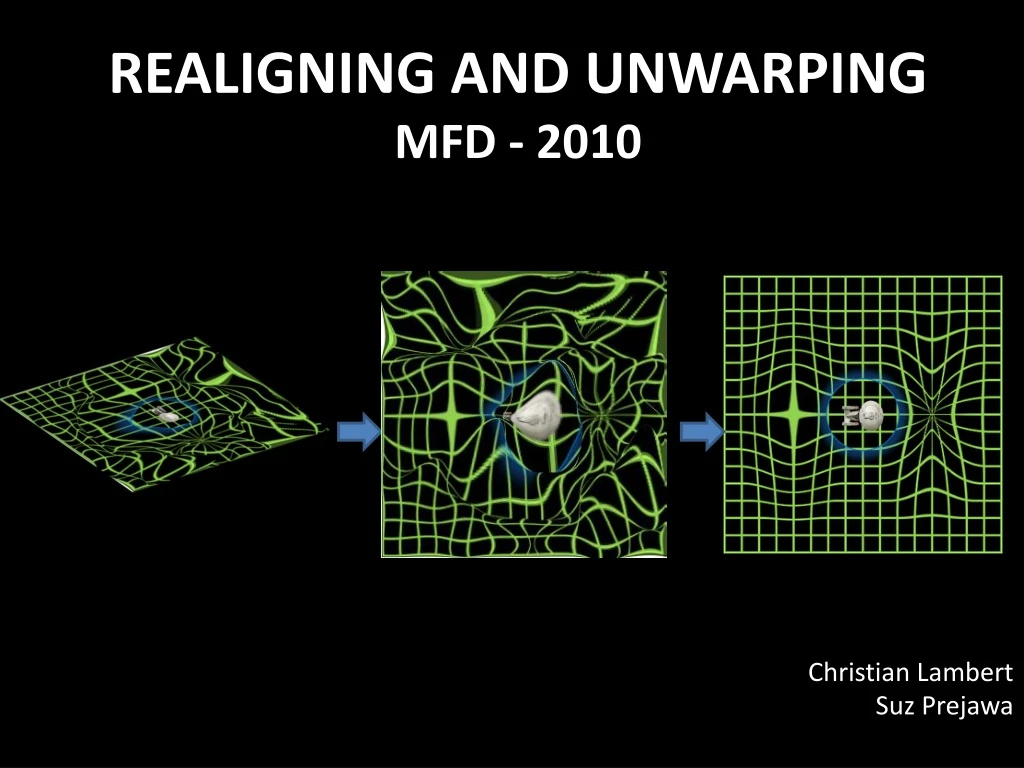
Christian Lambert Realigning and Unwarping MfD - 2010 • SuzPrejawa
Overview of SPM Analysis Statistical Parametric Map Design matrix General Linear Model Parameter Estimates fMRI time-series MotionCorrection Smoothing SpatialNormalisation Anatomical Reference
Overview • Motion in fMRI • Motion Prevention • Motion Correction • Realignment – Two Steps • Registration • Transformation • Realignment in SPM • Unwarping
Motion in fMRI • We want to compare the same part of the brain across time • Subjects move in the scanner • Even small head movements can be a major problem: • Movement artefacts add up to the residual variance and reduce sensitivity • Data may be lost if sudden movements occur during a single volume • Movements may be correlated with the task performed • Minimising movements is one of the most important factors for ensuring good data quality
Motion Prevention in fMRI • Constrain the volunteer’s head (soft padding) • Give explicit instructions to lie as still as possible, not to talk between sessions, and swallow as little as possible • Try not to scan for too long* – everyone will move after while! • Make sure your subject is as comfortable as possible before you start.
Realignment - Two Steps • Realignment (of same-modality images from same subject) involves two stages: • Registration • Estimate the 6 parameters that describe the rigid body transformation between each image and a reference image • 2. Transformation • Re-sample each image according to the determined transformation parameters
1. Registration • Each transform can be applied in 3 dimensions • Therefore, if we correct for both rotation and translation, we will compute 6 parameters Rotation Translation Z Yaw Roll Y Pitch X
Rigid body transformations parameterised by: Rollabout Y axis Yaw about Z axis Pitchabout X axis Translations 1. Registration • Operations can be represented as affine transformation matrices: • x1 = m1,1x0 + m1,2y0 + m1,3z0 + m1,4 • y1 = m2,1x0 + m2,2y0 + m2,3z0 + m2,4 • z1 = m3,1x0 + m3,2y0 + m3,3z0 + m3,4
Realignment - Two Steps • Realignment (of same-modality images from same subject) involves two stages: • Registration • Estimate the 6 parameters that describe the rigid body transformation between each image and a reference image • 2. Transformation • Re-sample each image according to the determined transformation parameters
2. Transformation • Reslice a series of registered images such that they match the first image selected onto the same grid of voxels • Various methods of transformation / interpolation: • Nearest neighbour • Linear interpolation • B-Spline
Simple Interpolation • Nearest neighbour • Takes the value of the closest voxel • Tri-linear • Weighted average of the neighbouring voxels • f5 = f1 x2 + f2 x1 • f6 = f3 x2 + f4 x1 • f7 = f5 y2 + f6 y1
B-spline Interpolation A continuous function is represented by a linear combination of basis functions 2D B-spline basis functions of degrees 0, 1, 2 and 3 B-splines are piecewise polynomials B-spline interpolation with degrees 0 and 1 is the same as nearest neighbour and bilinear/trilinear interpolation.
Residual Errors in Realigned fMRI Even after realignment a considerable amount of the variance can be accounted for by effects of movement • This can be caused by e.g.: • Movement between and within slice acquisition • Interpolation artefacts due to resampling • Non-linear distortions and drop-out due to inhomogeneity of the magnetic field • Incorporate movement parameters as confounds in the statistical model
References • SPM Website - www.fil.ion.ucl.ac.uk/spm/ • SPM 8 Manual - www.fil.ion.ucl.ac.uk/spm/doc/manual.pdf • MfD 2007 slides • SPM Course Zürich2008 - slides by Ged Ridgway • SPM Short Course DVD 2006 • John Ashburner’s slides - www.fil.ion.ucl.ac.uk/spm/course/slides09/
UNWARPING Has nothing to do with Star Trek’s warp engines… SuzPrejawa
No correction tmax=13.38 Pre-processing- what’s the point? To reduce the introduction of false positives in your analysis
Get a move on!…when movement makes life difficult • In extreme cases, up to 90% of the variance in fMRI time-series can be accounted for by effects of movement after realignment. • This can be due to non-linear distortion from magnetic field inhomogeneities
Magnetic Field Inhomogeneities- II Different tissues have different magnetic susceptibilities distortions in magnetic field distortions are most noticeable near air-tissue interfaces (e.g. OFC and anterior MTL) Field inhomogeneities have the effect that locations on the image are ‘deflected’ with respect to the real object Field inhomogeneity is measured in parts per million (ppm) with respect to the external field
Why is that important? … Non-rigid deformation … • Knowing the location at which 1H spins will precess at a particular frequency and thus where the signal comes from is dependent upon correctly assigning a particular field strength to a particular location. • If the field B0 is homogeneous, then the image is sampled according to a regular grid and voxels can be localised to the same bit of brain tissue over subsequent scans by realigning, this is because the same transformation is applied to all voxels between each scan. • If there are inhomogeneities in B0, then different deformations will occur at different points in the field over different scans, giving rise to non-rigid deformation. B0Expect field strength to be B0 here, so H atoms with signal associated with resonant frequency ω0 to be located here. In fact, because of inhomogeneity, they are here.
Data can help with your data 1) The image we obtain is a distorted image 2) There will be movements within the scanner.
Data can help with your data! The movements interact with the distortions. Therefore changes in the image as a result of head movements do not really follow the rigid body assumption: the brain may not alter as it moves, but the images do.
Susceptibility-by-motion interactions • Field inhomogeneities change with the position of the object in the field, so there can be non-rigid, as well as rigid distortion over subsequent scans. • The movement-by-inhomogeneity interaction can be observed by changes in the deformation field* over subsequent scans. A deformation field indicates the directions and magnitudes of location deflections throughout the magnetic field (B0) with respect to the real object. Vectors indicating distance & direction The amount of distortion is proportional to the absolute value of the field inhomogeneity and the data acquisition time.
So here comes the good news! With a FIELDMAP you can unwarp your scans (SPM toolbox!) a fieldmap measures field inhomogeneity (potentially per every scan) captures deformation field find the derivatives of the deformations with respect to subject movement for every scan, how exactly did my data warp/ how much did the deformation field change? igl.stanford.edu/~torsten/ct-dsa.html
Unwarp can estimate changes in distortion from movement Resulting field map at each time point Measured field map Estimated change in field wrt change in pitch (x-axis) Estimated change in field wrt change in roll (y-axis) 0 0 = + + • Using: • distortions in a reference image (FieldMap) • subject motion parameters (that we obtain in realignment) • change in deformation field with subject movement (estimated via iteration) • To give an estimate of the distortion at each time point.
Measure deformation field (FieldMap). Estimate new distortion fields for each image: estimate rate of change of the distortion field with respect to the movement parameters. Unwarp time series Estimate movement parameters +
Applying the deformation field to the image • Once the deformation field has been • modelled over time, the time-variant • field is applied to the image. • effect of sampling a regular object over a curved surface. • The image is therefore re-sampled • assuming voxels, corresponding to • the same bits of brain tissue, occur • at different locations over time.
The outcome? • In the end what you get is resliced copies of your images (with the letter ‘u’ appended to the front) that have been • realigned (to correct for subject movement) and • unwarped (to correct for the movement-by-distortion interaction) accordingly*. • These images are then taken forward to the next preprocessing steps (next week!). *NB. You can ‘realign’ and ‘unwarp’ separately if you prefer.
All very well, but how do I actually do this? • In scanner: acquire 1 set of fieldmaps for each subject • After scanning: convert fieldmaps into .img files (DICOM import in SPM menu) • Use fieldmap toolbox to create .vdm (voxel displacement map) files for each run for each subject. * You need to enter various default values in this step, so check physics wiki for what’s appropriate to your scanner type and scanning sequence 4. Enter vdm* files with EPI images into ‘realign + unwarp step’. This realigns your images and unwarps them in one step.
Series number Step 2: fieldmap toolbox on SPM8 • If using toolbox, you need to load the right phase and mag images. • phase: one for which there’s only one file with that series number • Mag: the first file of the two files with the same series number
Realign + unwarp in spm8 Click ‘RUN’ • Click on ‘new session’ as many times as your session numbers • ‘images’ = EPI data fM*.img, ~100s images • ‘phase map’ = vdm*.img • Do this for each session • The rest is probably default • Same goes for ‘Unwarp and reslicing options’
So hopefully you understand that... Tissue differences in the brain distort the signal, giving distorted images As the subject moves, the distortions vary Therefore images do not follow the rigid-body assumption. Unwarp estimates how these distortions change as the subject moves
No correction Correction by covariation Correction by Unwarp tmax=13.38 tmax=9.57 tmax=5.06 Advantages of incorporating this in pre-processing • One could include the movement parameters as confounds in the statistical model of activations. • However, this may remove activations of interest if they are correlated with the movement.
Practicalities Unwarp is of use when variance due to movement is large. Particularly useful when the movements are task related as can remove unwanted variance without removing “true” activations. Can dramatically reduce variance in areas susceptible to greatest distortion (e.g. orbitofrontal cortex and regions of the temporal lobe). Useful when high field strength or long readout time increases amount of distortion in images. Can be computationally intensive… so take a long time
References Jezzard, P. and Clare, S. 1999. Sources of distortion in functional MRI data. Human Brain Mapping, 8:80-85 Andersson JLR, Hutton C, Ashburner J, Turner R, Friston K (2001) Modelling geometric deformations in EPI time series. Neuroimage 13: 903-919 Previous years MfD slides. John Ashburner’s slides http://www.fil.ion.ucl.ac.uk/spm/course/#slides This ppt: www.fil.ion.ucl.ac.uk/~mgray/Presentations/Unwarping.ppt Physics WIKI SPM website/ SPM manual And Chloe Hutton.