Download
1 / 30
300 likes | 478 Views
Realigning and Unwarping MfD - 2009. Idalmis Santiesteban Karen Hodgson. Overview of SPM Analysis. Statistical Parametric Map. Design matrix. General Linear Model. Parameter Estimates. fMRI time-series. Motion Correction. Smoothing.

E N D
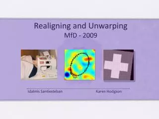
Realigning and Unwarping MfD - 2009 Idalmis Santiesteban Karen Hodgson
Overview of SPM Analysis Statistical Parametric Map Design matrix General Linear Model Parameter Estimates fMRI time-series MotionCorrection Smoothing SpatialNormalisation Anatomical Reference
Overview • Motion in fMRI • Motion Prevention • Motion Correction • Realignment – Two Steps • Registration • Transformation • Realignment in SPM • Unwarping
Motion in fMRI • We want to compare the same part of the brain across time • Subjects move in the scanner • Even small head movements can be a major problem: • Movement artefacts add up to the residual variance and reduce sensitivity • Data may be lost if sudden movements occur during a single volume • Movements may be correlated with the task performed • Minimising movements is one of the most important factors for ensuring good data quality
Motion Prevention in fMRI • Constrain the volunteer’s head • Give explicit instructions to remain as calm as possible, not to talk between sessions, and swallow as little as possible • Do not scan for too long – everyone will move after while!
Realignment - Two Steps • Realignment (of same-modality images from same subject) involves two stages: • Registration • Estimate the 6 parameters that describe the rigid body transformation between each image and a reference image • 2. Transformation • Re-sample each image according to the determined transformation parameters
1. Registration • Each transform can be applied in 3 dimensions • Therefore, if we correct for both rotation and translation, we will compute 6 parameters Rotation Translation Z Yaw Roll Y Pitch X
Rigid body transformations parameterised by: Rollabout Y axis Yaw about Z axis Pitchabout X axis Translations 1. Registration • Operations can be represented as affine transformation matrices: • x1 = m1,1x0 + m1,2y0 + m1,3z0 + m1,4 • y1 = m2,1x0 + m2,2y0 + m2,3z0 + m2,4 • z1 = m3,1x0 + m3,2y0 + m3,3z0 + m3,4
Realignment - Two Steps • Realignment (of same-modality images from same subject) involves two stages: • Registration • Estimate the 6 parameters that describe the rigid body transformation between each image and a reference image • 2. Transformation • Re-sample each image according to the determined transformation parameters
2. Transformation • Reslice a series of registered images such that they match the first image selected onto the same grid of voxels • Various methods of transformation / interpolation: • Nearest neighbour • Linear interpolation • B-Spline
Simple Interpolation • Nearest neighbour • Takes the value of the closest voxel • Tri-linear • Weighted average of the neighbouring voxels • f5 = f1 x2 + f2 x1 • f6 = f3 x2 + f4 x1 • f7 = f5 y2 + f6 y1
B-spline Interpolation A continuous function is represented by a linear combination of basis functions 2D B-spline basis functions of degrees 0, 1, 2 and 3 B-splines are piecewise polynomials B-spline interpolation with degrees 0 and 1 is the same as nearest neighbour and bilinear/trilinear interpolation.
Residual Errors in Realigned fMRI Even after realignment a considerable amount of the variance can be accounted for by effects of movement • This can be caused by e.g.: • Movement between and within slice acquisition • Interpolation artefacts due to resampling • Non-linear distortions and drop-out due to inhomogeneity of the magnetic field • Incorporate movement parameters as confounds in the statistical model
Unwarping Non-linear distortions due to inhomogeneities in the magnetic field
Why we need unwarp... • Realignment deals with any linear shifts • But after realignment there are still significant levels of variance resulting from subject movement within the scanner. • These will reduce the sensitivity to detect “true” activations especially if movements correlate with the task (e.g. speech etc)
Image distortions • The image that you acquire is a distorted image of the object in the scanner. • This is because the magnetic field is affected by differences in tissue composition across the brain • The image is particularly distorted at air-tissue interfaces (so orbitofrontal cortex and the regions of the temporal lobe). • The level of distortion can be increased with higher readout times (e.g. in higher resolution sequences) and higher field strengths . • This is important as severe distortions can lead to signal loss.
Deformation fields • To model the distortions in a single image, you can use a deformation field.
For an undistorted image.... • In SPM you can use the FieldMap toolbox to model this deformation field. Raw EPI Undistorted EPI
However the distortions vary with movement • The image we obtain is a distorted image • There will be movements within the scanner. • The movements interact with the distortions. • Therefore changes in the image as a result of head movements do not really follow the rigid body assumption: the brain may not alter as it moves, but the images do.
To demonstrate... • Distortions vary with the object position • Original vs rotated deformation vectors vary • Linear translation of rotated onto original: non-rigid body.
So given that distortions vary as the subject moves, how can we correct for motion artefacts? UNWARP
Unwarp can estimate changes in distortion from movement • Using: • distortions in a reference image (FieldMap) • subject motion parameters (that we obtain in realignment) • change in deformation field with subject movement (estimated via iteration) • To give an estimate of the distortion at each time point. Resulting field map at each time point Measured field map Estimated change in field wrt change in pitch (x-axis) Estimated change in field wrt change in roll (y-axis) 0 0 = + +
Measure deformation field (FieldMap). Estimate new distortion fields for each image: estimate rate of change of the distortion field with respect to the movement parameters. Unwarp time series Estimate movement parameters +
So hopefully you understand that... • Tissue differences in the brain distort the signal, giving distorted images • As the subject moves, the distortions vary • Therefore images do not follow the rigid-body assumption. • Unwarp estimates how these distortions change as the subject moves
Practicalities • Unwarp is of use when variance due to movement is large. • Particularly useful when the movements are task related as can remove unwanted variance without removing “true” activations. • Can dramatically reduce variance in areas susceptible to greatest distortion (e.g. orbitofrontal cortex and regions of the temporal lobe). • Useful when high field strength or long readout time increases amount of distortion in images.
References • SPM Website - www.fil.ion.ucl.ac.uk/spm/ • SPM 8 Manual - www.fil.ion.ucl.ac.uk/spm/doc/manual.pdf • MfD 2007 slides • SPM Course Zürich2008 - slides by Ged Ridgway • SPM Short Course DVD 2006 • John Ashburner’s slides - www.fil.ion.ucl.ac.uk/spm/course/slides09/