Download
1 / 65
650 likes | 825 Views
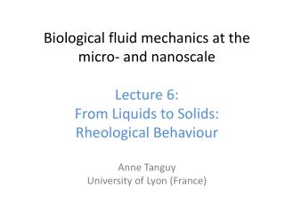
Biological fluid mechanics at the micro‐ and nanoscale Lecture 6: From Liquids to Solids : Rheological Behaviour Anne Tanguy University of Lyon (France). From Liquids to Solids : Rheological behaviour Elastic Solid Plastic Flow Visco - elasticity Non- Linear rheology.

E N D
Biological fluid mechanics at the micro‐ and nanoscale Lecture 6: FromLiquids to Solids: RheologicalBehaviour Anne Tanguy University of Lyon (France)
FromLiquids to Solids: • Rheologicalbehaviour • ElasticSolid • Plastic Flow • Visco-elasticity • Non-Linearrheology
Al polycristal (Electron Back Scattering Diffraction) Dendritic growth in Al: Cu polycristal : cold lamination (70%)/ annealing. TiO2 metallic foams, prepared with different aging, and different tensioactif agent: Si3N4 SiC dense
Whatis a « continuous » medium? • Two close elementsevolvein a similarway. • In particular: conservation of proximity. • « Field » = physicalquantityaveraged • over a volume element. • = continuousfunction of space. • Hypothesisin practice, to bechecked. • Atthisscale, forces are short range (surface forces between volume elements) In general, itisvalidatscales>>characteristicscalein the microstructure. Examples:crystals d >> interatomic distance (~ Å ) polycrystals d >> grain size (~nm ~mm) regularpacking of grains d >> grain size (~ mm) liquids d >> mean free path disorderedmaterials d >> 100 interatomic distances (~10nm)
REMINDER: The Navier-Stokes equation: with for a « Newtonian fluid » Thus: for an incompressible, Newtonian fluid. (h dynamical viscosity) The case of an Elastic Solid: No transport of matter, displacement field u Stress is related to the Strain Hooke’s Law: (anisotropy) 21 Elastic Moduli Cijlk in a 3D solid. Thus: for a Linear Elastic Solid
(1635-1703) 1678: Robert Hooke develops his “True Theory of Elasticity” Ut tensio, sic vis (ceiii nosstuv) “The power of any spring is in the same proportion with the tension thereof.” Hooke’s Law: τ = G γ or (Stress = G x Strain) where G is the RIGIDITY MODULUS
Example of an homogeneous and isotropic medium: F 2 Elastic Moduli (l,m) E, Young modulus n, Poisson ratio u Hydrostatic compression: Traction: Simple Shear: m, shear modulus P c, compressibility.
Sound waves in an isotropic medium: 2 sound wave velocities cL and cT Onde longitudinale: Le mouvement des atomes est dans le sens de la propagation Onde longitudinale: Ondes transverses: simple shear Onde transverse: Le mouvement des atomes est perpendiculaire au sens de la propagation
Examples of anisotropicmaterials (crystals): The number of Elastic Moduli depends on the Symetry Ex. cobalt Co: HC FCC T=450°C 3 moduli (3 equivalent axis) HCP 5 moduli C11 C12 C13 C33 C44 C66=(C11-C12)/2 FCC 3 moduli C11 C12 C44 6 (5) moduli (rotational invariance around an axis)
Voigt notation: 21 independent Elastic Moduli
Microscopic expression for the local ElasticModuli: Simple example of a cubiccrystal. On each bond: strain stress Elastic Modulus
General case: Local Elastic Moduli at small strain Born-Huang C1 ~ 2 m1 C2 ~ 2 m2 C3 ~ 2 (l+m) Example of an amorphous material Progressive convergence to an isotropic material at large scale M. Tsamados et al. (2007) 2D Lennard-Jones Glass N=216 225 L=483
Plastic Flow: F S F/S u Lz Plastic Flow Elasticité E u/Lz vitreloy In the Linear Elastic Regime: F/S = E.u/Lz Elasticity + Viscoelasticity Strain e Compressive stress s Plastic Threshold sy Visco-plastic Flow sflow ( e ) . Elastic modulus
Rheological Description of the Plastic Flow: Rheological law: shear stress at a given P and T, as a function of shear strain, strain rate. Creep experiment: at a constant t, what is e(t)? Relaxation exp.: at a constant e, what is t(t)? (here: t(t)=m.e if e<tY /m and t(t)=tY else) Apparent viscosity: h(t,e,de/dt) = t (t,e,de/dt) / (de/dt) (here: h=∞ if e<tY /m and h=0 else) Here, no temporal dependence (≠ viscous flow)
Example: Flow due to an external force (cf. Poiseuille flow) Binary Lennard-Jones Glass at T=0.2<Tg for tW=104 LJ F. Varnik (2008) Not a Poiseuille Flow atsmall T (Visco-Plastic) Poiseuille ≠Poiseuille
(1643-1727) 1687: Isaac Newton addresses liquids and steady simple shearing flow in his “Principia” “The resistance which arises from the lack of slipperiness of the parts of the liquid, other things being equal, is proportional to the velocity with which the parts of the liquid are separated from one another.” Newton’s Law: τ = η dγ/dt where η is the Coefficient of Viscosity Newtonian
Different behaviours: Newtonian Viscous Fluid: Ex. Water, honey.. Kelvin-VoigtSolid: Delayed Elasticity (anelastic behaviour). Maxwell Fluid: Ex. Solid close to TfInstantaneous Elasticity + Viscous Flow GeneralLinear Visco-Elastic Behaviour:
Dynamical Rheometers: Oscillatory forcing: Response: G’, Storage (Elastic) Modulus Instantaneous response G’’, Loss (Viscous) Modulus Delay Example of Perfect Elastic Solid: Example of Newtonian Viscous Fluid: Example of Maxwell Fluid:
Energy Balance: Elastic Energy Stored during T/4 And then given back (per unit volume and unit time). Averaged Dissipated Energy per unit time, during T/4, due to viscous friction >0 Loss Factor (Internal Friction)
Viscoelasticity of Polymers: General features amorphous crystalline Storage Modulus Internal Friction
Viscoelasticity of Mineral Glasses: Examples SiO2 – Na2O Si– Al-O-N Lekki et al.
Viscoelasticity and crystallization Mineral Glass ZrF4 Polymer (PET) Cristallization: G’ increases, mobility decreases
Frequency dependent behaviour SiO2-Na20-Ca0
Example of Blood Red Cells: e(t)/t0 G’ G’’
Creep MetalsCeramics Polymers T > 0,3-0,4 Tm 0,4-0,5 Tm Tg Macroscopic creep in Metals: ~ 1h Dislocation creep: b=0 m=4-6 Non-Linear behaviour 0.3 Tm<T<0.7 Tm Nabarro-Herring creep: b=2 m=1 Linear (Newtonian) flow diffusion of defects T>0.7 Tm Lead Romanian Pipe Metling Temperatures, for P=1 atm, Ice: Tm=273°K, Lead: Tm=600°K, Tungsten: Tm=3000°K
Theoretical Limit Athermal Elastic Limit Core Volume Elasticity Grain Boundaries Volume 10-1 Plasticity 10-2 Creep Dislocation 10-3 10-4 Creep Diffusion 10-5 10-6 0 0,3 0,5 0,7 1
Pastes Colloids Powders Metallic Glass Mineral Glass (SiO2, a-Si) Polymers (PMMA,PC)
From the Liquid to the Amorphous Solid: Non-Linear Rheological Behaviour F. Varnik (2006) 3D Lenard-Jones Glass
Non-Linear Rheological Behaviours: Shear softening Ex. painting, shampoo Shear thickening Ex. wet sand, polymeric oil, silly-putty Plastic Fluid Ex. amorphous solids, pastes
Example: in amorphous systems (glasses, colloids..) with b<1 Ex. Beads made of polyelectric gel shear softening Ex. Lennard-Jones Glass Tsamados, 2010
Simulations of Rheological Behaviour at constant Strain Rate and Temperature in an amorphous glassy material (Lennard-Jones Glass) Low strain rate Progressive Diffusion of Local Rearrangements Finite Size Effects Large strain rate Nucleation of Local Rearrangements M. Tsamados 2010
Density of nucleating centers per unit strain Diffusion of plasticity Cooperativity Maximum when L1=L2
Lecture 7 • AtomisticModelling: • ClassicalMolecular Dynamics Simulations • for fluiddynamics. • Description • The example of Wetting • The example of ShearDeformation
Classical Molecular Dynamics Simulations consists in solving the Newton’s equations for an assembly of particles interacting through an empirical potentiaL; In the Microcanonical Ensemble (Isolated system): Total energy E=cst In the Canonical Ensemble: Temperature T=cst with if no external force Different possible thermostats: Rescaling of velocities, Langevin-Andersen, Nosé-Hoover… more or less compatible with ensemble averages of statistical mechanics.
Equations of motion: the example of Verlet’s algorithm. Adapt the equations of motion, to the chosen Thermostat for cst T.
Thermostats: after substracted the Center of Mass velocity, or the Average Velocity along Layers • Langevin Thermostat: • Random force k(t) • Friction force –G.v(t) with <k(t).k(t’)>=cste.2GkBT.d(t-t’) • Andersen Thermostat: prob. of collision nDt, Maxwell-Boltzman velocity distr. • Nosé-Hoover Thermostat: • Rescaling of velocities: • Berendsen Thermostat: with • Heat transfer. Coupling to a heat bath. ( )1/2
Examples of Empirical Interactions: The Lennard-Jones Potential: 2-body interactions cf. van der Waals Length scales sij ≈ 10 Å Masses mi≈10-25 kg Energy eij≈ 1 eV ≈ 2.10-19J ≈ kBTm Time scale or Time step Dt = 0.01t ≈ 10-14 s 106 MD steps ≈ 10-8 s = 10 ns or 106x10-4=100% shear strain in quasi-static simulations N=106 particles, Box size L=100s ≈ 0.1 mm for a mass density r=1. 3.N.Nneig≈108 operations at each « time » step.
The Stillinger-Weber Potential: For « Silicon » Si, with 3-body interactions Stillinger-Weber Potential F. Stillinger and T. A. Weber, Phys. Rev. B31 (1985) Melting T Vibration modes Structure Factor The BKS Potential: For Silica SiO2, with long range effective Coulombian Interactions B.W.H. Van Beest, G.J. Kramer and R.A. Van Santen, Phys. Rev. Lett.64 (1990) Ewald Summation of the long-range interactions, or Additional Screening (Kerrache 2005, Carré 2008) 2-body interactions (Cauchy Model) 3-body interactions
Example: Melting of a Stillinger-Weber glass, from T=0 to T=2.
Microscopic determination of different physical quantities: • Density profile, pair distribution function • Velocity profile • Diffusion constant • Stress tensor (Irwin-Kirkwood, Goldenberg-Goldhirsch) • Shear viscosity (Kubo)