SDSS Analysis: Redshift, Spectra, LSS and Distributions
Explore the analysis of the Sloan Digital Sky Survey (SDSS) covering redshift space distortions, photometric surveys, correlations, and data releases. Learn about sample selection, photometric redshifts, and SDSS current status. Discover the power spectrum, angular correlations, and adaptive template methods used in the study.

SDSS Analysis: Redshift, Spectra, LSS and Distributions
E N D
Presentation Transcript
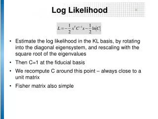
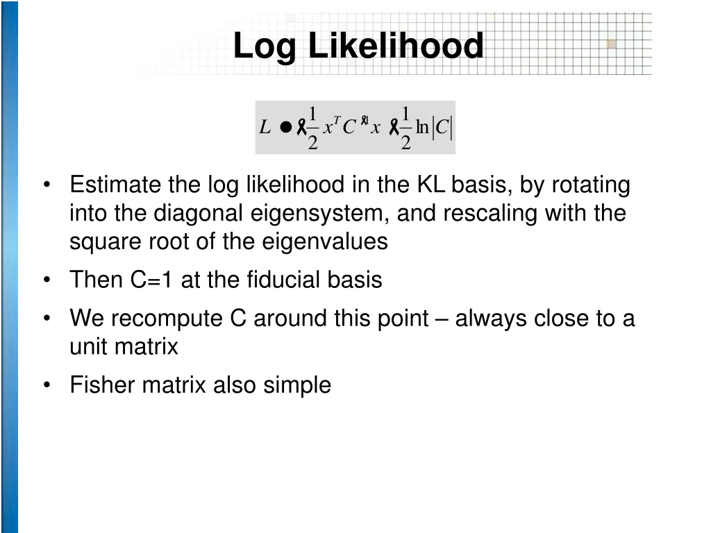
Log Likelihood • Estimate the log likelihood in the KL basis, by rotating into the diagonal eigensystem, and rescaling with the square root of the eigenvalues • Then C=1 at the fiducial basis • We recompute C around this point – always close to a unit matrix • Fisher matrix also simple
Quadratic Estimator • One can compute the correlation matrix of • P is averaged over shells, using the rotational invariance • Used widely for CMB, using the degeneracy of alm’s • Computationally simpler • But: includes 4th order contributions – more affected by nonlinearities • Parameter estimation is performed using
Distance from Redshift • Redshift measured from Doppler shift • Gives distance to zeroth order • But, galaxies are not at rest in the comoving frame: • Distortions along the radial directions • Originally homogeneous isotropic random field,now anisotropic!
Redshift Space Distortions Three different distortions • Linear infall (large scales) • Flattening of the redshift space correlations • L=2 and L=4 terms due to infall (Kaiser 86) • Thermal motion (small scales) • ‘Fingers of God’ • Cuspy exponential • Nonlinear infall (intermediate scales) • Caustics (Regos and Geller)
Power Spectrum • Linear infall is coming through the infall induced mock clustering • Velocities are tied to the density via • Using the continuity equation we get • Expanded: we get P2() and P4() terms • Fourier transforming:
r Angular Correlations • Limber’s equation
Applications • Angular clustering on small scales • Large scale clustering in redshift space
The Sloan Digital Sky Survey Special 2.5m telescope, at Apache Point, NM 3 degree field of view Zero distortion focal plane Two surveys in one Photometric survey in 5 bands detecting 300 million galaxies Spectroscopic redshift survey measuring 1 million distances Automated data reduction Over 120 man-years of development (Fermilab + collaboration scientists) Very high data volume Expect over 40 TB of raw data About 2 TB processed catalogs Data made available to the public
Current Status of SDSS • As of this moment: • About 4500 unique square degrees covered • 500,000 spectra taken (Gal+QSO+Stars) • Data Release 1 (Spring 2003) • About 2200 square degrees • About 200,000+ unique spectra • Current LSS Analyses • 2000-2500 square degrees of photometry • 140,000 redshifts
w() with Photo-z T. Budavari, A. Connolly, I. Csabai, I. Szapudi, A. Szalay, S. Dodelson,J. Frieman, R. Scranton, D. Johnston and the SDSS Collaboration • Sample selection based on rest-frame quantities • Strictly volume limited samples • Largest angular correlation study to date • Very clear detection of • Luminosity dependence • Color dependence • Results consistent with 3D clustering
ugriz L Type z Photometric Redshifts • Physical inversion of photometric measurements! Adaptive template method (Csabai etal 2001, Budavari etal 2001, Csabai etal 2002) • Covariance of parameters
343k 316k 254k 185k 280k 127k 326k 185k The Sample All: 50M mr<21 : 15M 10 stripes: 10M 0.1<z<0.3 -20 > Mr 2.2M 0.1<z<0.5 -21.4 > Mr 3.1M -20 > Mr >-21 1182k -21 > Mr >-23 931k -21 > Mr >-22 662k -22 > Mr >-23 269k
The Stripes • 10 stripes over the SDSS area, covering about 2800 square degrees • About 20% lost due to bad seeing • Masks: seeing, bright stars
The Masks • Stripe 11 + masks • Masks are derived from the database • bad seeing, bright stars, satellites, etc
The Analysis • eSpICE : I.Szapudi, S.Colombi and S.Prunet • Integrated with the database by T. Budavari • Extremely fast processing: • 1 stripe with about 1 million galaxies is processed in 3 mins • Usual figure was 10 min for 10,000 galaxies => 70 days • Each stripe processed separately for each cut • 2D angular correlation function computed • w(): average with rejection of pixels along the scan • Correlations due to flat field vector • Unavoidable for drift scan
Angular Correlations I. • Luminosity dependence: 3 cuts -20> M > -21 -21> M > -22 -22> M > -23
Angular Correlations II. • Color Dependence 4 bins by rest-frame SED type
Power-law Fits • Fitting
Bimodal w() • No change in slope with L cuts • Bimodal behavior with color cuts • Can be explained, if galaxy distribution is bimodal (early vs late) • Correlation functions different • Bright end (-20>) luminosity functions similar • Also seen in spectro sample (Glazebrook and Baldry) • In this case L cuts do not change the mix • Correlations similar • Prediction: change in slope around -18 • Color cuts would change mix • Changing slope
Redshift distribution • The distribution of the true redshift (z), given the photoz (s) • Bayes’ theorem • Given a selection window W(s) • A convolution with the selection window
Detailed modeling • Errors depend on S/N • Final dn/dz summed over bins of mr
Inversion to r0 From (dn/dz) + Limber’s equation => r0
Redshift-Space KL Adrian Pope, Takahiko Matsubara, Alex Szalay, Michael Blanton, Daniel Eisenstein, Bhuvnesh Jainand the SDSS Collaboration • Michael Blanton’s LSS sample 9s13: • SDSS main galaxy sample • -23 < Mr < -18.5, mr < 17.5 • 120k galaxy redshifts, 2k degrees2 • Three “slice-like” regions: • North Equatorial • South Equatorial • North High Latitude
Pixelization • Originally: 3 regions • North equator: 5174 cells, 1100 modes • North off equator: 3755 cells, 750 modes • South: 3563 cells, 1300 modes • Likelihoods calculated separately, then combined • Most recently: 15K cells, 3500 modes • Efficiency • sphere radius = 6 Mpc/h • 150 Mpc/h < d < 485 Mpc/h (80%): 95k • Removing fragmented patches: 70k • Keep only cells with filling factor >74%: 50k
Redshift Space Distortions • Expand correlation function • cnL = Skfk(geometry)b k • b = W0.6/b redshift distortion • b is the bias • Closed form for complicated anisotropy=> computationally fast
Wb/Wm Shape Wmh = 0.25 ± 0.04 fb = 0.26 ± 0.06 Wmh
b s8 Both depend on b b = 0.40 ± 0.08 s8 = 0.98 ± 0.03
Parameter Estimates • Values and STATISTICAL errors: Wh = 0.25 ± 0.05 Wb/Wm= 0.26 ± 0.06 b = 0.40 ± 0.05 s8 = 0.98 ± 0.03 • 1s error bars overlap with 2dF Wh = 0.20 ± 0.03 Wb/Wm = 0.15 ± 0.07 With h=0.71 Wm = 0.35 b = 1.33 s8m = 0.73 Degeneracy: Wh = 0.19 Wb/Wm= 0.17 also within 1s With h=0.7 Wm = 0.27 b = 1.13 s8m = 0.86 WMAP s8m = 0.84
Technical Challenges • Large linear algebra systems • KL basis: eigensystem of 15k x 15k matrix • Likelihood: inversions of 5k x 5k matrix • Hardware / Software • 64 bit Intel Itanium processors (4) • 28 GB main memory • Intel accelerated, multi-threaded LAPACK • Optimizations • Integrals: lookup tables, symmetries, 1D numerical • Minimization techniques for likelihoods
Systematic Errors • Main uncertainty: • Effects of zero points, flat field vectors result in large scale, correlated patterns • Two tasks: • Estimate how large is the effect • De-sensitize statistics • Monte-Carlo simulations: • 100 million random points, assigned to stripes, runs, camcols, fields, x,y positions and redshifts => database • Build MC error matrix due to zeropoint errors • Include error matrix in the KL basis • Some modes sensitive to zero points (# of free pmts) • Eliminate those modes from the analysis => projectionStatistics insensitive to zero points afterwards
SDSS LRG Sample • Three redshift samples in SDSS • Main Galaxies • 900K galaxies, high sampling density, but not very deep • Luminous Red Galaxies • 100K galaxies, color and flux selected • mr < 19.5, 0.15 < z < 0.45, close to volume-limited • Quasars • 20K QSOs, cover huge volume, but too sparsely sampled • LRGs on a “sweet spot” for cosmological parameters: • Better than main galaxies or QSOs for most parameters • Lower sampling rate than main galaxies, but much more volume (>2 Gpc3) • Good balance of volume and sampling
LRG Correlation Matrix • Curvature cannot be neglected • Distorted due to the angular-diameter distance relation (Alcock-Paczynski) including a volume change • We can still use a spherical cell, but need a weighting • All reduced to series expansions and lookup tables • Can fit for WL or w! • Full SDSS => good constraints • b and s8 no longer a constant b = b(z) = W(z)0.6 / b(z) • Must fit with parameterized bias model, cannot factor correlation matrix same way (non-linear)
Fisher Matrix Estimators • SDSS LRG sample • Can measureWLto ± 0.05 • Equation of state:w = w0 + z w1 Matsubara & Szalay (2002)
Summary • Large samples, selected on rest-frame criteria • Excellent agreement between redshift surveysand photo-z samples • Global shape of power spectrum understood • Good agreement with CMB estimations • Challenges: • Baryon bumps, cosmological constant, equation of state • Possible by redshift surveys alone! • Even better by combining analyses! • We are finally tying together CMB and low-z