Coaxial Architecture
Coaxial Architecture. Tree-and-Branch Architecture. Express Trunk. HFC Architecture. HUBS. node. Tap. Customer Homes. Businesses amp in building. Rural Network. Other cable outputs. Fiber Optic. Cable RF. (Node) Optics RX/TX. Headend. Active Device. Near Passive Network.

Coaxial Architecture
E N D
Presentation Transcript
Tree-and-Branch Architecture Express Trunk
HFC Architecture HUBS node Tap Customer Homes Businesses amp in building
Rural Network Other cable outputs Fiber Optic Cable RF (Node)Optics RX/TX Headend Active Device
Near Passive Network Two-Way Tap Eight-Way Tap Directional Coupler Splitter 11 26 14 29 Headend or Node 29 Optics RX/TX 17 24 21 LPI Four-Way Tap LPS
Passive Network 17 23 20 29 26 11 Two Way Tap Four Way Tap Slope Equalizer 17 Headend or Node Node 4
Sample Headend 1 Analog Video Com21 55-550 MHz splitter 2 Way RF out 430MHz 2 Way HCX comController DT 815 Amp RF splitter 2 5008ET2 3 EDFA Hub Public switch EDFA 2RRX HUB Return TX 2RRX DWDD Return TX DWDM
Connector Parts Body Boot Ferrule
Types of Connectors FC ST Biconic D4 SC
Coaxial Plant Designand Operation Optical Transmitters and Receivers
Topics • Overview • Optical Transmitters • Optical Receivers • Units of Optical Power • Power Budget
Optical Transmitter and Receiver Reproduced Electrical Signal Input ElectricalSignal Optical Signal Optical Fiber Transmitter Receiver
Optical Transmitter Drive Level Control Drive Level Test Point RF Input Optical Fiber Optical Connector Laser
Laser Drive Levels Clipped Output Laser Performance Curve Modulated Optical Output Optical Output Power Current Threshold Current Input RF Bias Current
Optical Receiver Bias Voltage Fiber Optical Connector Test Point Photo Detector RF Out Pre Amp Post Amp
Optical Power Equations dBm = 10 log mW mW = inverse log (dBm/10)
+/-10dB Optical Power Table Optical Power (dBm)Optical Power (mW) 30 1,000 20 100 10 10 0 1 -10 0.1 -20 0.01 -30 0.001
Power Budget Formula P b = T p - Rin where P b = the Power Budget T p = output Power of the Transmitter and R in = required input to the receiver
Optical Node System RF out NOR NRT
Optical Node Operation Post Amp H L 20 dBmV Post Amp H Pre Amp L Post Amp H L H L Node/Amplifier Block Diagram -20 dB Rf TP Light to RF Converter Splitter Level Control Tilt Generator Attenuator RF to Light Converter to RF Post Amp Combiner
Forward Optical Receivers/NOR’S RF Gain adjust 9A pad Optical monitoring T/P -30 down Test Point Optical alarm
Diamond Net RF Module
Coaxial Plant Designand Operation Amplifier Technology
Topics • Semiconductor Configurations in CATV • Single - Ended Amplifier • Push - Pull Amplifier • Parallel - Hybrid Amplifier
Single - Ended Amplifier 2nd Harmonic plus Noise
Parallel - Hybrid Amplifier Push Pull Stage Push Pull Stage Pin Pout ADVANTAGES: High Gain and Reduced Distortions
Coaxial Plant Designand Operation Amplifier Configurations
Objectives • Describe the most common amplifier configurations and discuss their usage. • Identify the components for each of the amplifier configuration and explain their functions and importance.
Amplifier Output Tilt 11dB of tilt @ 750 MHz
Attenuator Function 20 dBmV 20 dBmV 10 dBmV 10 dBmV 0 dBmV 0 dBmV 750 MHz 750 MHz 50 MHz 50 MHz
Equalizer Function Effect of Cable 20 dBmV 10 dBmV 10 dBmV 0 dBmV 750 MHz 50 MHz Combined Results 0 dB 750 MHz 50 MHz 10 dB Effect of Equalizer 20 dB 750 MHz 50 MHz
Response Equalizer Examples of Peak to Valley Responses. With Response Equalizers Installed These are available in either bumps or traps
Equalizer Selection 20 dB 11 dB Interstage Eq Set for desired Tilt @ Output Secondary Eq Set Additional Tilt 12 dB 50 MHz 750 MHz 11 dB = = = 8 dB 62E750/11 50 MHz 750 MHz
DC TP High Low Post Amp Pad Input EQ ALSC Optional Plug In Input Atten Interstage Slope Eq. Manual Gain Adj. Response Equalizer Interstage Atten. Inter Stage Amp Pre Amp Dist EQ High High DC TP Pad Low Low Shorting Stub to One Secondary or DC 4-8-or 12 Post Amp High DC TP Low Amplifier Block Diagram withALSC / AGC
Forward Sweep SYSTEM AMPLIFIER SWEEP GEAR METER
Sweep System Requirements Fiber Optic Interconnect Headend Combiner Fiber Transmitter Sweep Transmitter Node AMP 1 Reference Amp 4 Amp 2 Amp 3 Amp 5 Amp 6 *The remaining amplifiers in the cascade are compared to the reference.
Raw Sweep AFTER BEFORE
Coaxial Plant Designand Operation Frequency Response Specifics
Non Linear Cable Loss Characteristics Cable Kinks Z Mismatch Ideal Response Signal Level Signal Level 550MHz 50 MHz 550MHz 50 MHz Non Linear
Hardware Points of Concern Amplifier Connector Tap Cable Cable Cable Connector