Download
1 / 15
150 likes | 406 Views
Effects of the Great American Solar Eclipse on the lower ionosphere observed with VLF waves. Rok Vogrinčič University of Ljubljana, Slovenia Faculty of Mathematics and Physics ISWIW 2019, Trieste, 23.5.2019. Contents. Introduction Experimental setup The Great American Solar Eclipse

E N D
Effects of the Great American Solar Eclipse on the lower ionosphere observed with VLF waves Rok Vogrinčič University of Ljubljana, Slovenia Faculty of Mathematics and Physics ISWIW 2019, Trieste, 23.5.2019
Contents • Introduction • Experimental setup • The Great American Solar Eclipse • VLF observations • The box model • The Eclipse Model • Flare Input • Conclusion
Alejandro Lara Andrea Borgazzi Jean Pierre Raulin Source: http://www.geofisica.unam.mx/, https://www.facet.unt.edu.ar/ and https://www.mackenzie.br/centro-de-radio-astronomia-e-astrofisica-mackenzie/.
Introduction • Propagation of very low frequency (VLF) radio signals within the Earth-Ionosphere wave-guide is mainly affected by the solar UV. • Day/night variation or solar flares. • Ionospheric D-region at 70-80 km altitude; Ly-α radiation ionizes molecular and atomic species in the Earth’s atmosphere. • During a solar eclipse the effective height of the reflecting ionospheric layer rises (~5 – 10 km). Source: (top)https://sidstation.loudet.org/ionosphere-en.xhtml, (bottom) Hunsucker R. D., Hargreaves J. K.: The High-Latitude Ionosphere and its effects on Radio Propagation. Cambridge University Press, 2003.
Experimental setup • Latin America Very Low Frequency Network at Mexico (LAVNet-Mex) receiver station. • Location: 19°20’ N, 99°11’ W. • Detects changes in phase and amplitude of the VLF waves. • 100 turns, alu-frame with 1.8 m side, effective area ~ 324 m2. • BW = 40 kHz, f0 = 30 kHz, G = 51.88 dB, CMRR = 74.8 dB. • GPS receiver → 1 PPS signal → locking to GPS internal clock → signal phase with Δϕ < 1°. Source: Borgazzi, A., Lara, A., Paz, G., Raulin, J.P., The Ionosphere and the Latin America VLF Network Mexico (LAVNet-Mex) Station, Advances in Space Research (2014).
The Great American Solar Eclipse ND, USA, f = 25.2 kHz 3007.15 km long propagation path Mexico City, Mexico
VLF Observations – The box model Day/night change ~20-30 km.25% of the total diurnal average phase change accounts for 5-8 km.
The Eclipse Model The Covered solar disk and the Matrix model • Model of the phase deviation during the eclipse. • Considering effects of equivalent shortening of the propagation path between transmitter and receiver, and increasing of the effective ionospheric reflection height. • Equation by Wait, (1959) and Deshpande and Mitra, (1972): • Transform into: • and rewrite to: • Relative change equals:
Flare Input • C3.0 flare reaching its maximum x-ray flux at 17:57 UT. • Study the response of ionosphere during eclipse conditions. • Compare the duration and shape of the Solar x-ray flux excess and the ionospheric effect through the VLF data → sharper profile. • Phase difference in strong accordance with the X-ray flux → increase in the effective recombination coefficient.
Flare Input • Propagation distance function d = d(t). • Ionospheric height profile z = z(t) = z0 + Δze(t). • Δϕ is the phase difference only caused by the C3.0 flare. • The flare-induced ionospheric height difference Δz= Δzf(t). • In agreement with similar study done by Chakrabarti et al. (2018) → KSTD receiving station in Tulsa, USA → measured the signal amplitude. • Numerically reproduced observed signal with LWPC and the Wait’s 2-component D-region ionospheric model.
Flare Input Source: Chakrabarti, S.K., Sasmal, S., Chakraborty, S., Basak, T., Tucker, R.L., Modeling D-Region Ionospheric Response of the Great American TSE of August 21, 2017 from VLF signal perturbation (2018).
Conclusion • Estimated the rise of the reflection height at the time of the eclipse via the measured phase deviation of the received signal from NDK transmitter. • First approach with a box model gave an estimate to a rise in reflection height of about 5-8 km. • Proposed a model to quantify the changes of the Moon shadow along the propagation path as a function of time → obtained a good measure of the reflection height over the whole eclipse time interval. • At the time of the eclipse totality (18:00 UT), the rise in reflection height was about 9.3 +/- 0.1 km. • Good agreement with the results from previous ground and rocket measurements. • Model of the C3.0 flare in very good accordance with the results of simulations reported in the literature. • Our results are remarkable due to the relative simplicity of our approach. • Use of this model to study the eclipsed ionosphere.