Textbook and Syllabus
Textbook and Syllabus. Textbook : “Linear System Theory and Design”, Third Edition, Chi- Tsong Chen, Oxford University Press, 1999. Syllabus : Chapter 1 : Introduction Chapter 2 : Mathematical Descriptions of Systems Chapter 3 : Linear Algebra

Textbook and Syllabus
E N D
Presentation Transcript
Textbook and Syllabus Textbook: “Linear System Theory and Design”, Third Edition, Chi-Tsong Chen, Oxford University Press, 1999. Syllabus: Chapter 1: Introduction Chapter 2: Mathematical Descriptions of Systems Chapter 3: Linear Algebra Chapter 4: State-Space Solutions and Realizations Chapter 5: Stability Chapter 6: Controllability and Observability Chapter 7: Minimal Realizations and Coprime Fractions Chapter 8: State Feedback and State Estimators Additional: Optimal Control
Multivariable Calculus Grade Policy • Final Grade = 10% Homework + 20% Quizzes + 30% Midterm Exam + 40% Final Exam + Extra Points • Homeworks will be given in fairly regular basis. The average of homework grades contributes 10% of final grade. • Homeworks are to be submitted on A4 papers, otherwise they will not be graded. • Homeworks must be submitted on time. If you submit late, < 10 min. No penalty 10 – 60 min. –20 points > 60 min. –40 points • There will be 3 quizzes. Only the best 2 will be counted. The average of quiz grades contributes 20% of the final grade. • Midterm and final exam schedule will be announced in time. • Make up of quizzes and exams will be held one week after the schedule of the respective quizzes and exams.
Multivariable Calculus Grade Policy • The score of a make up quiz or exam, upon discretion, can be multiplied by 0.9 (i.e., the maximum score for a make up is then 90). • Extra points will be given if you solve a problem in front of the class. You will earn 1, 2, or 3 points. • You are responsible to read and understand the lecture slides. I am responsible to answer your questions. Modern ControlHomework 4Ronald Andre00920170000821 March 2021No.1. Answer: . . . . . . . . • Heading of Homework Papers (Required)
Chapter 1 Introduction Classical Control and Modern Control Classical Control • SISO (Single Input Single Output) • Low order ODEs • Time-invariant • Fixed parameters • Linear • Time-response approach • Continuous, analog • Before 80s Modern Control • MIMO(Multiple Input Multiple Output) • High order ODEs, PDEs • Time-invariant and time variant • Changing parameters • Linear and non-linear • Time- and frequency response approach • Tends to be discrete, digital • 80s and after • The difference between classical control and modern control originates from the different modeling approach used by each control. • The modeling approach used by modern control enables it to have new features not available for classical control.
Chapter 1 Modeling Approach Laplace Transform Approach RLCCircuit Resistor Inductor Capacitor Input variables: • Input voltage u(t) Output variables: • Current i(t)
Chapter 1 Modeling Approach Laplace Transform Approach Current dueto input Current due toinitial condition • For zero initial conditions (v0 = 0, i0 = 0), where Transfer function
Chapter 1 Modeling Approach State Space Approach • Laplace Transform method is not effective to model time-varying and non-linear systems. • The state space approach to be studied in this course will be able to handle more general systems. • The state space approach characterizes the properties of a system without solving for the exact output. • Let us now consider the same RLC circuit and try to use state space to model it.
Chapter 1 Modeling Approach State Space Approach RLC Circuit State variables: • Voltage across C • Current through L • We now have two first-order ODEs • Their variables are the state variables and the input
Chapter 1 Modeling Approach State Space Approach • The two equations are called state equations, and can be rewritten in the form of: • The output is described by an output equation:
Chapter 1 Modeling Approach State Space Approach • The state equations and output equation, combined together, form the state space description of the circuit. • In a more compact form, the state space can be written as:
Chapter 1 Modeling Approach State Space Approach • The state of a system at t0 is the information at t0 that, together with the input u for t0 ≤ t < ∞, uniquely determines the behavior of the system for t ≥ t0. • The number of state variables = the number of initial conditions needed to solve the problem. • As we will learn in the future, there are infinite numbers of state space that can represent a system. • The main features of state space approach are: • It describes the behaviors inside the system. • Stability and performance can be analyzed without solving for any differential equations. • Applicable to more general systems such as non-linear systems, time-varying system. • Modern control theory are developed using state space approach.
Chapter 2 Mathematical Descriptions of Systems Classification of Systems • Systems are classified based on: • The number of inputs and outputs: single-input single-output (SISO), multi-input multi-output (MIMO), MISO, SIMO. • Existence of memory: if the current output depends on the current input only, then the system is said to be memoryless, otherwise it has memory purely resistive circuit vs. RLC-circuit. • Causality: a system is called causal or non-anticipatory if the output depends only on the present and past inputs and independent of the future unfed inputs. • Dimensionality: the dimension of system can be finite (lumped) or infinite (distributed). • Linearity: superposition of inputs yields the superposition of outputs. • Time-Invariance: the characteristics of a system with the change of time.
Chapter 2 Mathematical Descriptions of Systems Linear System • A system y(t) = f(x(t),u(t)) is said to be linear if it follows the following conditions: • If then • If and then • Then, it can also be implied that
Chapter 2 Mathematical Descriptions of Systems Linear Time-Invariant (LTI) System • A system is said to be linear time-invariant if it is linear and its parameters do not change over time.
Chapter 2 Mathematical Descriptions of Systems State Space Equations • The state equations of a system can generally be written as: are the state variables are the system inputs • State equations are built of nlinearly-coupled first-order ordinary differential equations
Chapter 2 Mathematical Descriptions of Systems State Space Equations • By defining: we can write State Equations
Chapter 2 Mathematical Descriptions of Systems State Space Equations • The outputs of the state space are the linear combinations of the state variables and the inputs: are the system outputs
Chapter 2 Mathematical Descriptions of Systems State Space Equations • By defining: we can write Output Equations
Chapter 2 Mathematical Descriptions of Systems Example: Mechanical System State variables: Input variables: • Applied force u(t) Output variables: • Displacementy(t) State equations:
Chapter 2 Mathematical Descriptions of Systems Example: Mechanical System • The state space equations can now be constructed as below:
Chapter 2 Mathematical Descriptions of Systems Homework 1: Electrical System • Derive the state space representation of the following electric circuit: Input variables: • Input voltage u(t) Output variables: • Inductor voltagevL(t)
Chapter 2 Mathematical Descriptions of Systems Homework1A: Electrical System • Derive the state space representation of the following electric circuit: Input variables: • Input voltage u(t) Output variables: • Inductor voltagevL(t)