Download
1 / 40
400 likes | 423 Views
Learn about the invention of the perceptron, the first neural network model that could learn to recognize and identify optical patterns, and its remarkable learning algorithm.

E N D
CS 4700:Foundations of Artificial Intelligence Prof. Carla P. Gomes gomes@cs.cornell.edu Module: Perceptron Learning (Reading: Chapter 20.5)
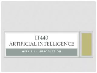
Rosenblatt & Mark I Perceptron: the first machine that could "learn" to recognize and identify optical patterns. Perceptron Cornell Aeronautical Laboratory • Perceptron • Invented by Frank Rosenblatt in 1957 in an attempt to understand human memory, learning, and cognitive processes. • The first neural network model by computation, with a remarkable learning algorithm: • If function can be represented by perceptron, the learning algorithm is guaranteed to quickly converge to the hidden function! • Became the foundation of pattern recognition research One of the earliest and most influential neural networks: An important milestone in AI.
Perceptron ROSENBLATT, Frank. (Cornell Aeronautical Laboratory at Cornell University ) The Perceptron: AProbabilistic Model for Information Storage and Organization in the Brain. In, Psychological Review, Vol. 65, No. 6, pp. 386-408, November, 1958.
Single Layer Feed-forward Neural NetworksPerceptrons • Single-layer neural network (perceptron network) A network with all the inputs connected directly to the outputs • Output units all operate separately: no shared weights Since each output unit is independent of the others, we can limit our study to single output perceptrons.
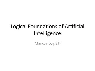
Seven line segments are enough to produce all 10 digits 2 1 3 0 6 4 5 Perceptron to Learn to Identify Digits(From Pat. Winston, MIT)
Seven line segments are enough to produce all 10 digits 2 1 3 0 6 4 5 Perceptron to Learn to Identify Digits(From Pat. Winston, MIT) A vision system reports which of the seven segments in the display are on, therefore producing the inputs for the perceptron.
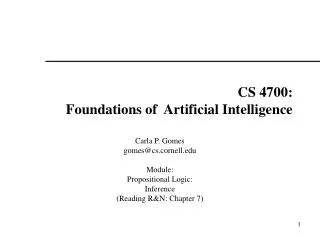
-1 0 0 Seven line segments are enough to produce all 10 digits 0 0 0 1 2 0 1 3 0 6 4 5 Perceptron to Learn to Identify Digit 0 When the input digit is 0, what’s the value of sum? Sum>0 output=1 Else output=0 A vision system reports which of the seven segments in the display are on, therefore producing the inputs for the perceptron.
Single Layer Feed-forward Neural NetworksPerceptrons Two input perceptron unit with a sigmoid (logistics) activation function: adjusting weights moves the location, orientation, and steepness of cliff
Perceptron Learning:Intuition • Weight Update • Input Ij (j=1,2,…,n) • Single output O: target output, T. • Consider some initial weights • Define example error: Err = T – O • Now just move weights in right direction! • If the error is positive, then we need to increase O. • Err >0 need to increase O; • Err <0 need to decrease O; • Each input unit j, contributes Wj Ij to total input: • if Ij is positive, increasing Wj tends to increase O; • if Ij is negative, decreasing Wj tends to increase O; • So, use: • Wj Wj + Ij Err • Perceptron Learning Rule (Rosenblatt 1960) is the learning rate.
Perceptron Learning:Simple Example • Let’s consider an example (adapted from Patrick Wintson book, MIT) • Framework and notation: • 0/1 signals • Input vector: • Weight vector: • x0 = 1 and 0=-w0, simulate the threshold. • O is output (0 or 1) (single output). • Threshold function: Learning rate = 1.
Intuitively correct, (e.g., if output is 0 but it should be 1, the weights are increased) ! Perceptron Learning:Simple Example Err = T – O Wj Wj + Ij Err • Set of examples, each example is a pair • i.e., an input vector and a label y (0 or 1). • Learning procedure, called the “error correcting method” • Start with all zero weight vector. • Cycle (repeatedly) through examples and for each example do: • If perceptron is 0 while it should be 1, • add the input vector to the weight vector • If perceptron is 1 while it should be 0, • subtract the input vector to the weight vector • Otherwise do nothing. This procedure provably converges (polynomial number of steps) if the function is represented by a perceptron (i.e., linearly separable)
Perceptron Learning:Simple Example • Consider learning the logical OR function. • Our examples are: • Sample x0 x1 x2 label • 1 1 0 0 0 • 2 1 0 1 1 • 3 1 1 0 1 • 4 1 1 1 1 Activation Function
w0 I0 I1 O w1 w2 I2 Perceptron Learning:Simple Example Error correcting method • If perceptron is 0 while it should be 1, • add the input vector to the weight vector • If perceptron is 1 while it should be 0, • subtract the input vector to the weight vector • Otherwise do nothing. 1 • We’ll use a single perceptron with three inputs. • We’ll start with all weights 0 W= <0,0,0> • Example 1 I= < 1 0 0> label=0 W= <0,0,0> • Perceptron (10+ 00+ 00 =0, S=0) output 0 • it classifies it as 0, so correct, do nothing • Example 2 I=<1 0 1> label=1 W= <0,0,0> • Perceptron (10+ 00+ 10 = 0) output 0 • it classifies it as 0, while it should be 1, so we add input to weights • W = <0,0,0> + <1,0,1>= <1,0,1>
w0 I0 I1 O w1 w2 I2 1 • Example 3 I=<1 1 0> label=1 W= <1,0,1> • Perceptron (10+ 10+ 00 > 0) output = 1 • it classifies it as 1, correct, do nothing • W = <1,0,1> • Example 4 I=<1 1 1> label=1 W= <1,0,1> • Perceptron (10+ 10+ 10 > 0) output = 1 • it classifies it as 1, correct, do nothing • W = <1,0,1>
w0 I0 I1 O w1 w2 I2 Perceptron Learning:Simple Example Error correcting method • If perceptron is 0 while it should be 1, • add the input vector to the weight vector • If perceptron is 1 while it should be 0, • subtract the input vector from the weight vector • Otherwise do nothing. 1 • Epoch 2, through the examples, W = <1,0,1> . • Example 1 I = <1,0,0> label=0 W = <1,0,1> • Perceptron (11+ 00+ 01 >0) output 1 • it classifies it as 1, while it should be 0, so subtract input from weights • W = <1,0,1> - <1,0,0> = <0, 0, 1> • Example 2 I=<1 0 1> label=1 W= <0,0,1> • Perceptron (10+ 00+ 11 > 0) output 1 • it classifies it as 1, so correct, do nothing
Example 3 I=<1 1 0> label=1 W= <0,0,1> • Perceptron (10+ 10+ 01 > 0) output = 0 • it classifies it as 0, while it should be 1, so add input to weights • W = <0,0,1> + W = <1,1,0> = <1, 1, 1> • Example 4 I=<1 1 1> label=1 W= <1,1,1> • Perceptron (11+ 11+ 11 > 0) output = 1 • it classifies it as 1, correct, do nothing • W = <1,1,1>
w0 I0 I1 O w1 w2 I2 Perceptron Learning:Simple Example 1 • Epoch 3, through the examples, W = <1,1,1> . • Example 1 I=<1,0,0> label=0 W = <1,1,1> • Perceptron (11+ 01+ 01 >0) output 1 • it classifies it as 1, while it should be 0, so subtract input from weights • W = <1,1,1> - W = <1,0,0> = <0, 1, 1> • Example 2 I=<1 0 1> label=1 W= <0, 1, 1> • Perceptron (10+ 01+ 11 > 0) output 1 • it classifies it as 1, so correct, do nothing
Example 3 I=<1 1 0> label=1 W= <0, 1, 1> • Perceptron (10+ 11+ 01 > 0) output = 1 • it classifies it as 1, correct, do nothing • Example 4 I=<1 1 1> label=1 W= <0, 1, 1> • Perceptron (10+ 11+ 11 > 0) output = 1 • it classifies it as 1, correct, do nothing • W = <1,1,1>
I0 I1 O W0 =0 I2 W1=1 W2=1 Perceptron Learning:Simple Example • Epoch 4, through the examples, W= <0, 1, 1>. • Example 1 I= <1,0,0> label=0 W = <0,1,1> • Perceptron (10+ 01+ 01 = 0) output 0 • it classifies it as 0, so correct, do nothing 1 OR So the final weight vector W= <0, 1, 1> classifies all examples correctly, and the perceptron has learned the function! Aside: in more realistic cases the bias (W0) will not be 0. (This was just a toy example!) Also, in general, many more inputs (100 to 1000)
Derivation of a learning rule for Perceptrons Minimizing Squared Errors • Threshold perceptrons have some advantages , in particular • Simple learning algorithm that fits a threshold perceptron to any • linearly separable training set. • Key idea: Learn by adjusting weights to reduce error on training set. • update weights repeatedly (epochs) for each example. • We’ll use: • Sum of squared errors (e.g., used in linear regression), classical error measure • Learning is an optimization search problem in weight space.
Derivation of a learning rule for Perceptrons Minimizing Squared Errors • Let S = {(xi, yi): i = 1, 2, ..., m} be a training set. (Note, x is a vector of inputs, and y is the vector of the true outputs.) • Let hw be the perceptron classifier represented by the weight vector w. • Definition:
Derivation of a learning rule for Perceptrons Minimizing Squared Errors • The squared error for a single training example with input x and true output y is: • Where hw (x) is the output of the perceptron on the example and y is the true output value. • We can use the gradient descent to reduce the squared error by calculating the partial derivatives of E with respect to each weight. Note: g’(in) derivative of the activation function. For sigmoid g’=g(1-g). For threshold perceptrons, Where g’(n) is undefined, the original perceptron rule simply omitted it.
Gradient descent algorithm we want to reduce , E, for each weight wi, change weight in direction of steepest descent: • Intuitively: • Err = y – hW(x) positive • output is too small weights are increased for positive inputs and decreased for negative inputs. • Err = y – hW(x) negative • opposite learning rate Wj Wj + Ij Err
Perceptron Learning:Intuition • Rule is intuitively correct! • Greedy Search: • Gradient descent through weight space! • Surprising proof of convergence: • Weight space has no local minima! • With enough examples, it will find the target function! • (provide not too large)
Gradient descent in weight space From T. M. Mitchell, Machine Learning
Epoch cycle through the examples Wj Wj + Ij Err • Perceptron learning rule: • Start with random weights, w = (w1, w2, ... , wn). • Select a training example (x,y) S. • Run the perceptron with input x and weights w to obtain g • Let be the training rate (a user-set parameter). • Go to 2. Epochsare repeated until some stopping criterion is reached— typically, that the weight changes have become very small. The stochastic gradient method selects examples randomly from the training set rather than cycling through them.