Download
1 / 23
230 likes | 247 Views
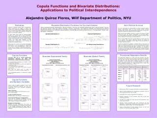
This presentation discusses the application of bivariate distributions in insurance, using mathematical techniques to address pricing and estimation problems. Includes numerical examples.

E N D
Insurance Applications of Bivariate Distributions David L. Homer & David R. Clark CAS Annual Meeting November 2003
AGENDA: • Explain the Insurance problem being addressed • Show the mathematical “machinery” used to address the problem • Provide a numerical example
AGENDA: • Explain the Insurance problem being addressed • Show the mathematical “machinery” used to address the problem • Provide a numerical example
The Players: Insured: Dietrichson Drilling A large account with predictable annual losses Insurer: Pacific All Risk Insurance Co. Actuary: You
The Pricing Problem: Pacific All-Risk Insurance Company sells a product that provides coverage on both • Specific Excess – individual losses above 600,000 • Aggregate Excess – above the sum of all retained losses capped at 3,000,000 in the aggregate
Policy Structure proposed for our insured Dietrichson Drilling 1,000,000 Per-Occurrence Layer 600,000 Per-occurrence Retained by the insured Stop Loss Layer 3,000,000 8,000,000 Aggregate Losses
How do we price this product? • Expected Losses are straight-forward • Expected Losses for the two coverages are additive • Separate distributions are straight-forward • A combined distribution is NOT
AGENDA: • Explain the Insurance problem being addressed • Show the mathematical “machinery” used to address the problem • Provide a numerical example
How do we estimate a single distribution? Define frequency and severity distributions, then: • Heckman-Meyers • Recursive methods (Panjer) • Simulation • Fast Fourier Transform (FFT)
Key Elements of FFT Technique: • Discretized severity vector x=(x0 ,…,xn-1) • FFT formula • IFFT formula
Convolution Theorem: The transform of the sum is equal to the product of the transforms. To sum up j independent identical variables:
Probability Generating Function: The PGFN is a short-cut method for combining the distributions for each possible number of claims. It does all of the convolutions for us!
Putting it all together we obtain the aggregate probability vector z from the severity probability vector x and the claim count PGFN :
Bivariate case is the same, but using a MATRIX instead of a VECTOR. becomes…
AGENDA: • Explain the Insurance problem being addressed • Show the mathematical “machinery” used to address the problem • Provide a numerical example
Pacific All-Risk: Severity Distribution Bivariate Severity Mx Single Claim Severity x Primary Excess Marginal 0 200,000 400,000 600,000 0 0.00% 0.00% 0.00% 0.00% 0.00% 200,000 37.80% 0.00% 0.00% 0.00% 37.80% 400,000 23.50% 0.00% 0.00% 0.00% 23.50% 600,000 14.60%9.10%15.00% 0.00% 38.70% 800,000 0.00% 0.00% 0.00% 0.00% 0.00% 1,000,000 0.00% 0.00% 0.00% 0.00% 0.00% Excess Marginal 75.90% 9.10% 15.00% 0.00% 100.00% 0 0.00% 200,000 37.80% 400,000 23.50% 600,000 14.60% 800,000 9.10% 1,000,000 15.00% Primary
Negative Binomial PGF for claim counts with Mean=5 and Variance=6:
Bivariate Aggregate Matrix Mz Excess 0 200,000 400,000 600,000 800,000 1,000,000 1,200,000 0 1.05% 0.00% 0.00% 0.00% 0.00% 0.00% 0.00% 200,000 1.65% 0.00% 0.00% 0.00% 0.00% 0.00% 0.00% 400,000 2.38% 0.00% 0.00% 0.00% 0.00% 0.00% 0.00% 600,000 3.09% 0.40% 0.66% 0.00% 0.00% 0.00% 0.00% 800,000 3.34% 0.65% 1.07% 0.00% 0.00% 0.00% 0.00% 1,000,000 3.39% 0.96% 1.58% 0.00% 0.00% 0.00% 0.00% 1,200,000 3.22% 1.27% 2.16% 0.26% 0.21% 0.00% 0.00% 1,400,000 2.86% 1.40% 2.44% 0.44% 0.36% 0.00% 0.00% 1,600,000 2.43% 1.45% 2.59% 0.66% 0.54% 0.00% 0.00% 1,800,000 1.97% 1.40% 2.57% 0.90% 0.78% 0.09% 0.05% 2,000,000 1.54% 1.26% 2.38% 1.02% 0.92% 0.15% 0.08% 2,200,000 1.17% 1.09% 2.12% 1.08% 1.01% 0.24% 0.13% 2,400,000 0.86% 0.90% 1.80% 1.08% 1.05% 0.33% 0.20% 2,600,000 0.62% 0.72% 1.47% 1.00% 1.01% 0.38% 0.24% 2,800,000 0.43% 0.55% 1.16% 0.88% 0.93% 0.42% 0.27% 3,000,000 0.29% 0.41% 0.89% 0.75% 0.82% 0.43% 0.29% Primary
Expected Per-Occurrence Loss = 391,000 overall = 830,334 in scenarios where stop loss is hit Both coverages go bad at the same time!
Other Applications: • Generation of Large & Small losses for DFA • Loss and ALAE with separate limits • Any other bivariate phenomenon (e.g., WC medical and indemnity)