
2. Physical Layer
E N D
Presentation Transcript
2. Physical Layer • 2.1 Definition • 2.2 Mechanical, ElectricalandFunctionalSpecifications • 2.3 Transmission Techniques, Modulation, Multiplexing • 2.4 Physical Media • 2.5 Example: DSL
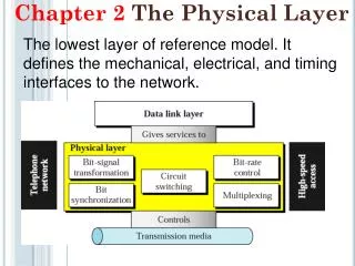
2.1 Definition of the Physical Layer • ISO-Definition • The physical layer defines mechanical, electrical, functional and pro-cedural properties, in order to establish, hold and tear downa physical connection between Data Terminal Equipment (DTE) and Data Circuit-Terminating Equipment (DCE). • The physical layer provides the transmission of a transparent bit stream between data link layer entities by physical connections. A physical con-nection may allow the transmission of a bit stream in duplex mode or half-duplex mode.
Properties of the Physical Layer • mechanical: Dimensions of connectors, assignment of pins, etc. e.g. ISO 4903: “Data Communication – 15 pin DTE/DCE interface connector and pin assignment” • electrical: Voltage levels, etc., e.g., CCITT X.27/V.11: “Electrical char-acteristics for balanced double-current interchange for gene-ral use with integrated circuit equipment in the field of data communication” • functional: Classification of functions (which pin has which function: data, control, timing, ground), e.g., CCITT X.24: “List of definitions for interchange circuits between DTE and DCE on public data networks” • procedural: Rules (procedures) for the use of the interface, e.g. CCITT X.21: “Interface between DTE and DCE for synchronous operation on public data networks”
2.2 Mechanical, Electrical and Functional Specifications • Mechanical Properties • Example: Ethernet UTPwith an RJ-45 connector • RJ45 is a standardized connector which specifies the physical male and female connectors as well as the pin assignments of the wires in a telephone cable. A UTP cable An RJ-45 connector pinassignment
Electrical Properties: CCITT V.28 (EIA RS-232-C) • For discrete electronic components • One conductor per circuit, plus a common ground for both directions • Bit rate limited to 20 kbit/s • Distance limited to 15 m • Produces substantial cross modulation
CCITT V.10/X.26 (EIA RS-423-A) • For IC components (integrated circuits) • One conductor per circuit, plus one common ground for each direction • Bit rate up to 300 kbit/s • Distance up to 1000 m at 3 kbit/s or up to 10 m at 300 kbit/s • Reduced cross modulation
CCITT V.11/X.27 (EIA RS-422-A) • For IC components (integrated circuits) • Two conductors per circuit • Bit rate up to 10 Mbit/s • Distance up to 1000 m at 100 kbit/s or up to 10 m at 10 Mbit/s • Minimal cross modulation
terminal network T (Transmit) DTE DCE C (Control) R (Receive) I (Indication) S (Signal Timing) B (Byte Timing) Ga (Common Return) G (Ground) Functional Properties • The functions of the X.21 pins
Functional/Procedural Specification in X.21 • (in analogy to the telephone)
location B location A Long-Distance Lines R (Receive) T (Transmit) DCE DTE DTE DCE C (Control) I (Indication) R (Receive) T (Transmit) I (Indication) C (Control) S (Signal Timing) S (Signal Timing) G (Ground) G (Ground) X.21 X.21 Local Interface vs. Long-Distance Line • The number of cables on the long-distance lines is not necessarily the same as the number of cables at the DCE/DTE interface!
Source Transformer Medium back-Transformer Primary Signal 2.3 Transmission Techniques, Modulation, Multiplexing Signal Transmission Example: analog signals in a telephone network • The primary signal (here acoustic) is converted by a transformer into an electrical (here analog) signal and converted back at the receiver. • From here on, we will assume that the primary signal on the source side is electrical, and the prim-ary signal on the receiver side is electrical as well. The transmission signal may also be electrical, with the same or other characteristics as the primary signal, but it may also be optical, a radio link, an infrared link, etc.
Signals • A signal is the physical representation of data. • Signal parameters are the physical characteristics of a signal that are used to represent the data. • For a time-dependend signal the value of the signal parameter S is a function of time: • S = S(t).
Classes of Signals (1) • Classification of time-dependent signals: • time-continuous, value-continuous signals • time-discrete, value-continuous signals • time-continuous, value-discrete signals • time-discrete, value-discrete signals • Is an exact signal value available at any given time? • yes: time-continuous • no: time-discrete • Are all signal values within a range of values permitted? • yes: value-continuous • no: value-discrete
time- continuous discrete s s continuous t t value- s s discrete t t Classes of Signals (2) Examples • value- and time-continuous: the analog telephone • value-continuous, time-discrete: a process control application with periodical measurements of analog values • value-discrete, time-continuous: continuous transmission of digital signal values • value- und time-discrete: digital values with a fixed sampling rate
Basic Transmission Techniques (1) • Digital input, digital transmission: digital line coding • Digital or analog input, analog transmission: modulation techniques • Analog input, digital transmission: Digitization, Pulse Code Modul-ation
analog: Amplifier digital: R Regenerator Basic Transmission Techniques(2) • Analog and Digital Transmission:
Digital Input, Digital Transmission • Modern digital transmission techniques use broadband techniques at very high bitrates (PCM technique, local area networks, etc.) • Desirable properties: • No DC component at the physical level • Recovery of the clock out of the arriving signal (self-clocking signal codes) • Detection of transmission errors already at the signal level • Signal Coding (Line Coding, Transmission Code): • The mapping of a digital data element to a (possibly different) digital signal element is called signal coding or line coding. The resulting time-discrete and value-discrete signal codes are called line codes or transmission codes.
Important Digital Line Codes (1) • Non-Return to Zero - Level (NRZ-L) • 1 = high voltage level 0 = low voltage level • Non-Return to Zero - Mark (NRZ-M) • 1 = transition at the beginning of the interval 0 = no transition at the beginning of the interval • Non-Return to Zero - Space (NRZ-S) • 1 = no transition at the beginning of the interval 0 = transition at the beginning of the interval • Return to Zero (RZ) • 1 = rectangular pulse at the beginning of the interval 0 = no rectangular pulse at the beginning of the interval
Important Digital Line Codes (2) • Manchester Code (Biphase Level) • 1 = transition from high to low in the middle of the interval 0 = transition from low to high in the middle of the interval • Biphase-Mark • Always a transition at the beginning of the interval. • 1 = another transition in the middle of the interval 0 = no transition in the middle of the interval • Biphase-Space • Always a transition at the beginning of the interval. • 1 = no transition in the middle of the interval 0 = another transition in the middle of the interval
Important Digital Line Codes (3) • Differential Manchester Code • Always a transition in the middle of the interval. • 1 = no transition at the beginning of the interval0 = additional transition at the beginning of the interval • Delay Modulation (Miller) • 1 = transition in the middle of the interval 0 = transition at the end of the interval only if followed by another 0 • Bipolar • 1 = rectangular pulse in the first half of the interval, alternating polarity0 = no rectangular pulse
Differential Line Codes • Differential Encoding: A signal difference (transition) encodes the value of the data bit. • NRZ-M (Mark), NRZ-S (Space) • NRZ-M: change of the signal value (transition to the opposite signal value) encodes a data value of “1“. • NRZ-S: change of the signal value encodes a data value of “0“. • Advantage over NRZ-L: On a noisy line signal changes are easier to detect than signal levels (which have to be compared with a threshold value). • Disadvantages of all NRZ codes: DC component and no clock signal bet-ween transmitter and receiver.
Biphase Codes • Biphase line codes have at least one signal change per bit interval and at most two signal changes per bit interval. • Advantages • Easy synchronisation (clocking) of the receiver since there is always a “pulse edge“ to trigger the receiver • No DC component in the signal • Some error detection at the signal level (physical level) possible: missing transitions can be recognized easily. • Disadvantage • Twice the number of rectangular pulses for the same bit rate! Requires a better line quality for the same bit rate.
Bit Rate and Baud Rate • Bit rate • Number of bits (binary data values) transmitted per second. • Baud rate • Number of rectangular pulses per second on the line.
Bipolar Code • The bipolar code is an example for a line coding with more than two signal values (here: a “tertiary“ signal). • The value “1“ is represented alternatingly by a positive or negative pulse in the first half of the bit interval. Therefore there is no DC component. • The bipolar code is also called AMI (Alternate Mark Inversion).
Digital/Analog Input, Analog Transmission • Modulation: encodes digital or analog input data on an analog carrier signal • Modem: Modulator-Demodulator • Example: transmission of digital data over the analog telephone network • Modulation methods • Amplitude Modulation (AM) • Frequency Modulation (FM) • Phase Modulation (PM)
Modulation Methods 1 1 0 0 1 1 0 0 • (a) Binary signal (bit stream) (b) Amplitude Modulation (AM) (c) Frequency Modulation (FM) (d) Phase Modulation (PM) Phase shift
o 45 amplitude phase shift o 15 (a) (b) Quadrature Amplitude Modulation • QAM (Quadrature Amplitude Modulation) is a combination of amplitude and phase modulation. Each point in the diagrams corresponds to a number of bits. • Two amplitudes, four phase change angles, eight data points, thus three bits transmitted per baud. Used in V.32 modems. • Sixteen data points, thus four bits transmitted per baud (used in V.32 modems for 9600 bit/s at 2400 baud)
Multiplexing • Transmission path • Physical transport system for signals (e.g., cable) • Transmission channel • Abstraction of a transmission path for a signal stream. • Often, multiple transmission channels are operated in parallel over one transmission path. The mapping of multiple channels on one path is called multiplexing.
frequency channel 1 channel 2 . . . channel n time Frequency Division Multiplexing • Broadband transmission paths allow the allocation of several transmission channels to different frequency bands: the available frequency range is sub-divided into a set of frequency bands, and a transmission channel is assig-ned to each band (frequency division multiplexing, FDM).
Channel 1 Channel 2 Channel 2 Channel 1 Channel 3 Attenuation factor Channel 3 frequency (HZ) (c) frequency (Hz) (a) carrier frequencies (kHz) (b) Frequency Division Multiplexing
Inter-channel gaps frequency ch 1 ch 2 ch 3 ch 4 ch 5 time Time Division Multiplexing • The entire available bandwidth is made available to one channel at a time, allowing very high baud rates. The channels take turns in accessing the phy-sical medium. Each channel receives one time slotper period (time divi-sion multiplexing, TDM).
Transmitter Receiver Synchronous Time Division Multiplexing • Time division multiplexing is applicable only to time-discrete signals (prefer-ably to time- and value-discrete signals = digital signals). With synchronous time division multiplexing, time is divided into fixed-size periods. Each of the n transmitters is assigned one time slot (time slice) TC1, TC2 .... TCn per period. Transmitters and detectors at the re-ceiver run at the same clock speed (in synch).
Direction of transmission content ch-id content ch-id content ch-id Asynchronous Time Division Multiplexing • The transmission path is not assigned to the transmitters in a static way but by need. Thus the receiver cannot derive the association of a piece of data with a channel from timing anymore. Therefore a channel id is now required for each data block (packet, cell). Asynchronous time division multiplexing is also called statistical time division multiplexing. With asynchronous TDM there is a statistical multi-plexing gain: the sum of the maximum rate of all data streams can be much higher than the bandwidth of the transmission path, as long as they do not all send at the same time at the maximum rate.
A2 A1 synchronous multiplexing 3 2 1 B1 C2 B1 C1 A2 A1 C2 C1 C2 B1 C1 A2 A1 asynchronous multiplexing Comparison of Multiplexing Methods
digital transmission system receiver transmitter analog signal analog signal analog-to- digital- conversion digital-to- analog- conversion digital signal Analog Input, Digital Transmission (1) • The transmission of analog data over a digital transmission paths requires the digitization of the data.
analog digital quantization value-continous value-discrete sampling time-continuous time-discrete Analog Input, Digital Transmission (2) • A/D- and D/A conversion for transmission of analog signals on digital trans-mission systems.
Advantages of Digital Transmission • Low error rate • nonoiseintroducedbyamplifiers • noaccumulationofnoiseoverlongdistances • Easier Time Division Multiplexing (TDM) • Digital circuitsareless expensive. • As a consequence, the digital storageandtransmissionof analog signalsbecomemoreandmorepopular: • audio on CD • video on DVD • DAB (Digital Audio Broadcast) • DVB (Digital Video Broadcast, digital TV) • andmanymore...
Sampling • In order to convert a time-continuous signal into a time-discrete signal, the input is sampled. • In most practical cases sampling is periodic.
Sampling Theorem of Nyquist • For an error-free reconstruction of the analog signal, a minimum sampling rate fA is necessary. The higher the frequencies in the analog data are, the higher the sampling frequency must be. For noise-free channels the Samp-ling Theorem of Nyquist applies: • Sampling Theorem • The sampling rate fA must be twice as high as the highest frequency in the signal fS: • fA = 2 * fS
a/2 a = size of the quantization interval a a/2 Quantization • The amplitude range of the analog signal is subdivided into a finite number of intervals (quantization intervals). To each interval a discrete value is as-signed. Since all analog signal values belonging to one quantization interval are assigned to the same discrete value, there will be a quantization error. Back transformation At the receiver the original analog value is reconstructed (digital-to-analog conversion). The maximum quantization error will be a/2.
Binary Encoding • Each quantization interval is represented by a binary value which is trans-mitted over the channel. • In many practical cases the binary representation is just the interval number.
Fundamental Quantization Trade-off • The finer the quantization interval, the smaller the quantization error, but the more bits we will need per sample. • In other words: the better the quality we need, the higher the bit rate will be.
signal value 7 6 5 4 3 2 1 0 001 010 101 011 110 101 111 100 time Sampling period Illustration of Sampling, Quantization and Encoding
analog analog PCM signal signal signal CODEC CODEC Pulse Code Modulation (PCM) • The combination of the steps • sampling • quantization • encoding • and the representation of the resulting bit stream as a digital baseband signal is called Pulse Code Modulation (PCM). • The A/D conversion (sampling, quantization and coding) as well as the D/A conversion is performed by a so-called CODEC (Coder/Decoder).
PCM Telephone Channels • The ITU-T (formerly CCITT) has standardized two PCM transmission sy-stems many years ago. • Starting point: the analog ITU-T telephone channel • Frequency band: 300 - 3400 Hz (range of human speech) • Bandwidth: 3100 Hz • Sampling rate: fA = 8 kHz • Sampling period: TA = 1/ fA = 1/8000 Hz = 125 µs • The sampling rate selected by the ITU-T is somewhat higher than necessary according to Nyquist’s sampling theorem: the maximum frequency of 3400 Hz would result in a sampling rate of 6800 Hz. There are technical reasons for the slightly higher sampling rate (noise, filter design, channel separation).
Amplitude Quantization • The number of quantization intervals was determined for speech commu-nication for good comprehensibility of syllables. The ITU-T considers 256 quantization intervals to be optimal (empirically determined). • For binary encoding these 256 intervals require 8 bits. • The transmission speed (bit rate) for a PCM telephone channel is thus: • Bit rate = sampling frequency times length of the codeword • kbit/s = 8000/s x 8 bits • = 64 kbit/s
Nonlinear Quantization (1) • With linear quantization, all intervals are equal in size and independent of the current value of the signal. • However, it turns out that humans perceive quantization errors (quantization noise)more clearly at small amplitudes. • With nonlinear quantization the quantization intervals are larger for large signal amplitudes and smaller for small amplitudes. • The nonlinear mapping is performed by a compressor which is inserted into the signal path upstream of the quantizer. On the receiving side an expanderinverts the operation. • Nonlinear quantization is usually based on a logarithmic curve. Technically, the mapping is approximated by linear sections in digital electronic circuits.
number of the quantization interval 113 … 128 - - 16 49 … 64 33 … 48 17 … 32 1_ - 1 - ½ ¼ ½ 1/8 1/16 1/32 standardized amplitude of the input signal Nonlinear Quantization (2) • 13-segment compressor curve