Download
1 / 76
760 likes | 863 Views
Explore tower-scale variability in CO2 flux across AmeriFlux sites, bridge temporal gaps, understand atmospheric CO2 mechanisms.

E N D
Merging CO2 flux and mixing ratio observations at synoptic, seasonal and interannual scales Kenneth J. Davis, Chuixiang Yi, Martha P. Butler, Michael D. Hurwitz and Daniel M. Ricciuto The Pennsylvania State University Peter S. Bakwin, NOAA CMDL Major contributions from the Walker Branch Watershed, Harvard Forest, Northern OBS and Little Washita sites, and the Fluxnet project
Goals Obtain a mechanistic understanding of tower-scale interannual variability in NEE of CO2 across many AmeriFlux/Fluxnet sites. + Link observations of interannual variability in tower fluxes with the global CO2 flask network. = Understand the mechanisms that govern interannual changes in the atmospheric CO2 budget.
Outline • Towards governing variables: (Yi et al) • Climatic factors and temporal variability in NEE at various time scales. • Temperature, drought and the light response of NEE. • Bridging the gap in scales: (Davis et al) • Examples of merging flux and concentration data at various time scales.
Part I: Climate variables and NEE at various time scales(NB, WB, WL, HF) Respiration and temperature Correlation between nighttime tower flux and air temperature is very high on daily, monthly and seasonal time scales. Correlation breaks down on interannual scales.
Respiration and temperature Northern OBS tower (NB) Manitoba, Canada Wofsy, Munger et al. Boreal black spruce forest
Respiration and temperature WLEF TV tower (WL) Northern Wisconsin, USA Davis, Bakwin et al. Mixed forest/wetland mosaic
Respiration and temperature Harvard Forest (HF) Massachusetts, USA Wofsy, Munger et al. Deciduous forest
Respiration and temperature Walker Branch tower (WB) Baldocchi, Wilson et al. Tennessee, USA Deciduous forest
Why does the temperature-respiration relationship break down on annual time scales? Hypotheses: • Annual respiration is proportional to annual litter production which is a weak function of temperature? • Temperature sensitivity is limited at the seasonal extremes (summer, winter).
Season NB B R2T WL B R2T HV B R2T WB B R2T Spring 0.0351 0.47 -5.1 0.0844 0.50 5.2 0.0445 0.38 5.1 0.0632 0.60 13.3 Summer 0.0676 0.36 13.3 0.0526 0.23 16.2 0.0255 0.08 17.0 0.0283 0.10 22.3 Autumn 0.0603 0.83 -1.3 0.0801 0.45 7.8 0.0231 0.18 8.0 0.0547 0.66 14.1 Winter 0.0126 0.08 -21.8 0.0142 0.04 -7.0 0.0283 0.08 -3.3 0.0340 0.46 4.4 Seasonal distribution of temperature sensitivity B, (Re=AeBT ). Spring B is the largest except at the NB site. There is no correlation between T and respiration in winter except at the WB site.
Climate variables and NEE at various time scales(NB, WB, WL, HF) NEE of CO2 and precipitation Correlation between NEE and precipitation is very poor on daily, monthly and seasonal time scales. Correlation becomes strong for interannual time scales.
NEE and precipitation Northern OBS tower (NB) Manitoba, Canada Wofsy, Munger et al. Boreal black spruce forest
NEE and precipitation WLEF TV tower (WL) Northern Wisconsin, USA Davis, Bakwin et al. Mixed forest/wetland mosaic
NEE and precipitation Harvard Forest (HF) Massachusetts, USA Wofsy, Munger et al. Deciduous forest
NEE and precipitation Walker Branch tower (WB) Baldocchi, Wilson et al. Tennessee, USA Deciduous forest
Climate variables and NEE at various time scales(NB, WB, WL, HF) NEE and net radiation Correlation between NEE and net radiation is strong on all time scales.
NEE and net radiation Northern OBS tower (NB) Manitoba, Canada Wofsy, Munger et al. Boreal black spruce forest
NEE and net radiation WLEF TV tower (WL) Northern Wisconsin, USA Davis, Bakwin et al. Mixed forest/wetland mosaic
NEE and net radiation Harvard Forest (HF) Massachusetts, USA Wofsy, Munger et al. Deciduous forest
NEE and net radiation Walker Branch tower (WB) Baldocchi, Wilson et al. Tennessee, USA Deciduous forest
Summary • Dependence of NEE on climatic factors is not consistent across time scales. • Net radiation and precipitation become more correlated with NEE on annual time scale. • Dryness=Rn/(L*P) may be used as an annual controlling parameter on interannual variability of NEE of CO2.
Discontinuous permafrost exists Water stress is not critical Soil thaw is critical; this depends on Rn Drought leads to more release of CO2 With abundant soil moisture, available energy is critical for CO2 uptake. As dryness>0.95, water stress becomes critical. 1998 is the second year of drought. 1999 is the third year of drought. (?) Drought has strong effect on interannual variability in NEE at WB. NB WL HV WB
Across many sites Average per site over several years HV-Harvard Forest (US,92-99) TH-Tharandt (Germany, 97-99) WL-WLEF (US, 97-99) WB-Walker Branch (US,95-98) NO-Norunda (Sweden,96-97) LW-Little Washita (US,97-98) LO-Loobos (Netherlands,97-98) HL-Howland (US, 96-97) HE-Hesse (France, 98-99)
Part II: Temperature, drought and light response of NEE(LW, WB, WL, HF) Drought and NEE Drought stress is evident. Diurnal asymmetry is intruiging.
How does drought stress modify the diurnal pattern of NEE with climate factors in the growing season? • Use multi-year daytime data in growing season (June-July-August) for each site to make diurnal average for NEE and climate variables. • Examine the relationship between NEE and climate variables. • Dry years are shown in red, and wet years in blue on the plots.
Walker Branch Plus-Morning; Circle-Afternoon Dotted line-AM; solid line-PM F=NEE; Q=PAR • 1) Drought stress effect • (mean =1995-1998, red=1995, blue=1998) • 2) Diurnal asymmetry? • Is AM different from PM? • -Plant experiences show: stomata opening is larger in AM, smaller in PM and near closed at midday. • -Stomata open in the light or in response to a low concentration of CO2, close in darkness or when dehydration causes a loss of turgor. • -Stomata open quickly and close slowly. • -The time lag between transpiration and tree water uptake is as much as 3 hours.
Grassland (LW, 1997, 1998, mean = 1996-1998) In a very dry year, no photosynthesis. High T limits respiration. Drought drives grass ecosystem from a carbon sink to a source
Water Use Efficiency WUE = NEE/LE In AM, wue decreases with T In PM, wue is small and almost constant. Drought reduces wue Wue is much smaller at WL and LW than at WB and HV
Part II: Temperature, drought and light response of NEE(LW, WB, WL, HF) Temperature and NEE Light response factors are functions of temperature.
F=NEE, Q=PAR F=F(T, VPD, Q, Rn) VPD=VPD(T) Rn=Rn(Q) F=F(T, Q)
Light response of ecosystem CO2 exchange R=canopy dark respiration, or total ecosystem respiration F¥=canopy assimilation rate at saturating light a=Apparent quantum yield Hypothesis: R, F¥and adepend on temperature. Method: Nonparametric statistical method. Data: Multi-year daytime flux data in growing season.
Isopleths of NEE in a (T, Q) plane Common features: Under high light conditions, temperature plays a key role in NEE and there is an optimal domain. Difference: In low light conditions, temperature also has an important impact on NEE at WL and LW, a smaller impact at HV, but no effect at WB.
Functions of T on R, F¥,and a. R(T) is expected F¥(T) at HV is different from WB. F¥(T) in AM is different from PM (WB). Higher T extremely reduces F¥ at WB. F¥ increases with T and saturates at higher T at HV. Water stress is critical at WB. Available energy is critical at HV. Global a is sensitive to T within specific range at WB. a is quite different between AM and PM.
Summary • Diurnal asymmetry of relationship between NEE and climate variables is observed clearly. • The light response of ecosystem CO2 exchange is affected by temperature and drought stress. • Maximum assimilation rate and apparent quantum yield are temperature-dependent.
Part III: Bridging the gap across regions to continents • Problem: Flux vs. mixing ratio observations – mismatch in scales. • Method: CO2 mixing ratios from flux towers • Application: What can we learn from a single site? • Advection matters • CO2 advection occurs with weather • ABL budget method is promising for regional fluxes • Joint analyses of CO2 – H2O may help. • Application: How can we integrate multiple sites? • Continental and regional network ideas • Spatial coherence across many sites – spring anomaly
Atmospheric approaches to observing the terrestrial carbon cycle Time rate of change (e.g. CO2) Mean transport Turbulent transport (flux) Source in the atmosphere Average over the depth of the atmosphere (or the ABL): F0C encompasses all surface exchange: Oceans, deforestation, terrestrial uptake, fossil fuel emissions. Inversion study: Observe C, model U, derive F Flux study: Observe F directly
Methods for determining NEE of CO2Methods for bridging the gap Upscale via ecosystem models and networks of towers. Move towards regional inverse modeling
Methodology: How can we use flux towers to gather worthwhile CO2 mixing ratio measurements? • Calibrate! Bakwin et al, 1995. Zhao et al, 1997. • Use midday data - very small vertical gradients. • Midday surface layer CO2 data resolves synoptic, seasonal and annual spatial and temporal trends.
Chequamegon Ecosystem-Atmosphere Study (ChEAS) http://cheas.psu.edu WLEF tall tower (447m) CO2 flux measurements at: 30, 122 and 396 m CO2 mixing ratio measurements at: 11, 30, 76, 122, 244 and 396 m Forest stand towers: Mature upland deciduous Deciduous wetland Mixed old growth All have both CO2 flux and high precision mixing ratio measurements.
North Upland, wetland, and very tall flux tower. Old growth tower to the NE. High-precision CO2 profile at each site. Mini-mesonet, 15-20km spacing between towers. Lost Creek Landcover key Open water WLEF Wetland Coniferous Mixed deciduous/coniferous Shrubland Willow Creek General Agriculture
Surface layer flux towers canbe used to monitor continental CO2!
The seasonal amplitude of the gradient in CO2 between the continental ABL and the marine boundary layer is large. Surface layer - mid-ABL difference (1 to 2 ppmv) does not overwhelm this signal.
Applications • Advection and local fluxes are both important in the ABL CO2 budget. • Relative importance changes across the continent. • Advection can be huge with synoptic events. • In between synoptic events, even 1-D ABL budgets do a fair job for flux estimates.